The IEEE 39-bus "New England" benchmark: 10 generators (red, sized by injected power), 29 load and junction buses (blue), 46 transmission lines. Every figure in this notebook is computed from this topology with the companion package KuramotoGrid`.
A power grid is a giant network of coupled oscillators. Each generator is a spinning mass that wants to turn at exactly 50 or 60-Hz; the transmission lines pull neighbouring machines into step. Whether the whole continent locks into a single rhythm – synchronisation – is the difference between keeping the lights on and a blackout. In this notebook we put the textbook Kuramoto model on the real IEEE 39-bus transmission topology, with the actual generation and load of the New England system. We watch synchronisation switch on as a function of the coupling strength, measure the stability margin of the physical operating point, and then run a full N-1 contingency screen to find the one line whose loss desynchronises the grid. We then turn the very same machinery on the real British National Grid (the reduced GB transmission model) and find its weakest corridor. We close on why the energy transition – less spinning inertia, differently-placed injections – makes all of this harder. Dynamical systems × critical infrastructure × the physics of the grid.
1. Setup
1. Setup
The whole analysis lives in one companion package, kuramoto_powergrid_helpers.wl, attached to this post. It carries the IEEE-39-bus data (taken verbatim from MATPOWER's case39), the network layout, and every model and plotting routine. Download it next to this notebook and evaluate the cell below; the core model cells then run directly. (A few cells in the live-data sections are shown as illustrative calls – with placeholder URLs/arguments – since the figures here are pre-rendered; the exact, runnable versions are in the wolfram/ scripts listed in the final section.)
SetDirectory[NotebookDirectory[]];Get["kuramoto_powergrid_helpers.wl"];
A quick sanity check on the data: 39 buses, 46 lines, and a net power injection vector that sums to zero (generation balances load once line losses are absorbed).
P=kgInjection[];(*per-unitnetinjection,100MVAbase*){Length[P],Length[kgBranches[]],Total[P]}
{39,46,1.07×}
-14
10
2. From spinning machines to the Kuramoto model
2. From spinning machines to the Kuramoto model
Every synchronous generator on the grid is a flywheel. Call the phase angle of machine i measured in a frame that co-rotates with the nominal grid frequency. If the machine runs exactly on frequency, is constant; if it speeds up or slows down, drifts. Newton's law for a rotating machine – the swing equation – balances inertia and damping against the net electrical power:
θ
i
θ
i
θ
i
M
i
..
θ
i
D
i
θ
i
P
i
∑
j
B
ij
θ
i
θ
j
Here is the inertia of the machine, its damping, and the net power it injects (generation minus local load). The sum is the power flowing out along each line to neighbour j: in the lossless ("DC power flow") approximation that power is sin(-), where = 1/ is the line susceptance and K is a global coupling dial. This is exactly the second-order Kuramoto model (Filatrella et al. 2008; Motter et al. 2013).
M
i
D
i
P
i
B
ij
θ
i
θ
j
B
ij
x
ij
Drop the inertia term (0) and you get the first-order Kuramoto model,
M
i
θ
i
P
i
∑
j
B
ij
θ
i
θ
j
whose phase-locked fixed points are precisely the lossless power-flow solutions of the grid. We use the first-order model to map out whether the grid can synchronise (Sections 5–7) and the full second-order model to watch how it does so in time (Sections 8–9).
The health of the synchronised state is summarised by the Kuramoto order parameter,
r=
ψ
1
N
∑
j
θ
j
a complex number whose magnitude r runs from 0 (phases scattered uniformly round the circle – incoherent) to 1 (all phases identical – perfect synchrony). For a grid with heterogeneous injections, even a perfectly frequency-locked state has r < 1, because the machines settle at different fixed phase offsets.
3. The IEEE 39-bus New England network
3. The IEEE 39-bus New England network
The IEEE 39-bus system is the standard medium-size benchmark for transient-stability studies – a reduced model of the New England transmission grid (Athay, Podmore & Virmani 1979). It has 39 buses, 46 lines and 10 generators carrying about 6.2GW of generation and load. We build it as a weighted graph, the edge weight of each line being its susceptance = 1/.
B
ij
x
ij
g=kgGraph[];kgNetworkPlot["PlotLabel"->"IEEE 39-bus topology"]
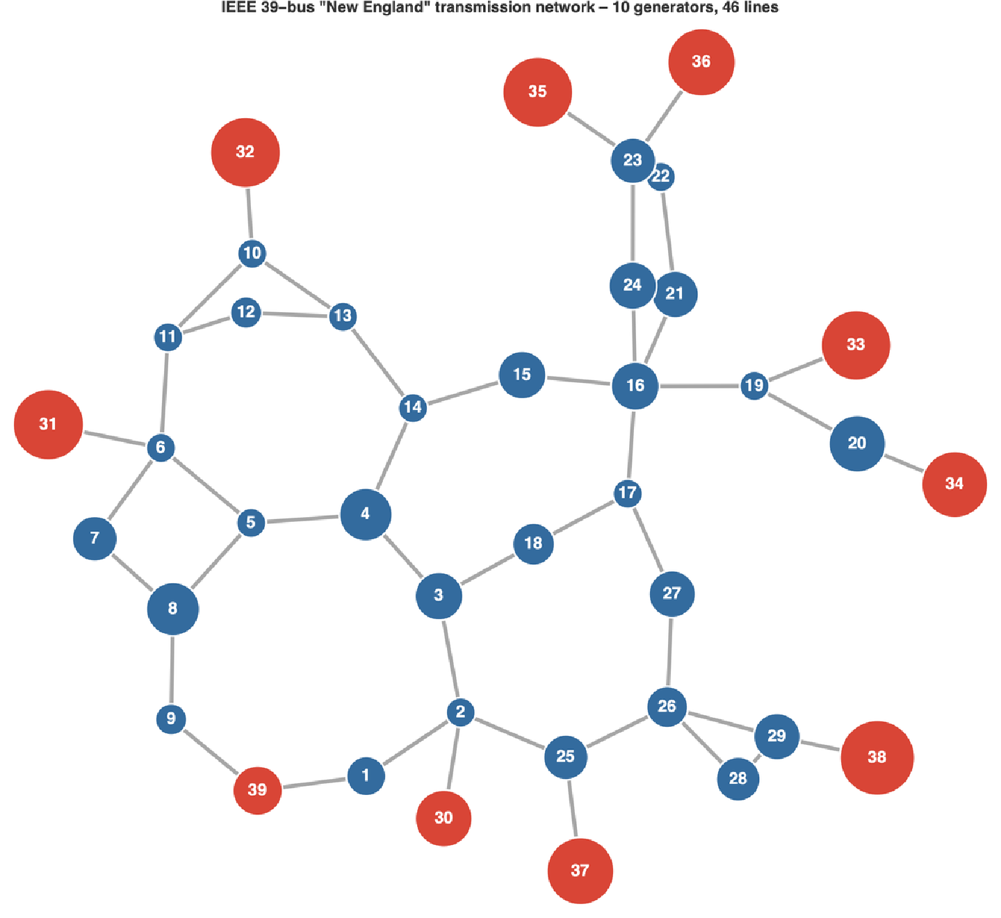
Generators sit on radial "stubs" (the step-up transformers 30–39); the meshed core carries the bulk transfers. Node area encodes the magnitude of the power injection – note the two largest machines, buses 38 (830MW) and 39 (the 1GW equivalent of the rest of the Eastern Interconnection).
The reactances span more than an order of magnitude, so the coupling between neighbours is strongly heterogeneous – some lines are far stiffer than others. That heterogeneity is exactly what makes one line, rather than another, the critical one.
4. The phase-locked operating point
4. The phase-locked operating point
At a given coupling K the grid's steady state solves the lossless power-flow equations = K ∑ sin(-). We solve them by Newton iteration, warm-started from the linearised (DC) solution using the weighted graph Laplacian L.
P
i
B
ij
θ
i
θ
j
θ=KP
+
L
fp=kgFixedPoint[1.0];(*K=1isthephysicalgrid*){fp["exists"],fp["maxAngle"]/Degree,kgOrderParameter[fp["theta"]][[1]]}
{True,9.61,0.996}
At the physical operating point the grid locks comfortably: the largest phase difference across any line is only about 9.6° (the static-stability limit is 90°), and the order parameter is 0.996. The grid is deep inside its stable basin – which is exactly how a real transmission system is operated.
5. Synchronisation as a function of coupling strength
5. Synchronisation as a function of coupling strength
Now turn the coupling dial. For each K we ask whether a stable phase-locked state exists and, if so, how coherent it is. Below a critical coupling the locked branch disappears in a saddle-node bifurcation and the machines drift out of step; above it the grid synchronises.
K
c
Kc=kgCriticalCoupling[{}]rK=Table[{K,kgOrderParameter[kgFixedPoint[K]["theta"]][[1]]},{K,Kc,2,0.05}];ListLinePlot[rK,Filling->Axis]
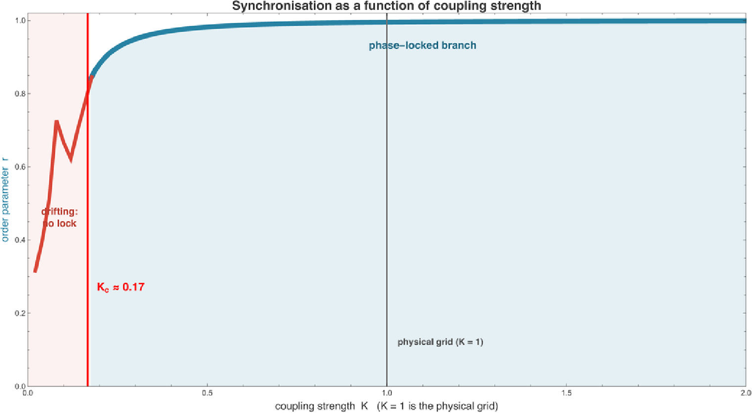
The synchronisation transition. The blue phase-locked branch (solid) exists only above ≈ 0.17; below it (red, from direct simulation) the grid drifts and the order parameter collapses. The physical grid operates at K = 1, well above . (The honest operating margin is the small phase angle across the most-loaded line, Section 6; lowering K is a modelling device – equivalent to scaling every injection up uniformly – not a direction a real grid actually moves in.)
K
c
K
c
Two animations make the transition tangible. The first is the classic Kuramoto picture made physical: each of the 39 machines is a point on the unit circle at its rotor angle, and the whole grid spins (shown slowed). Starting scattered and at rest, the machines swing – with real second-order inertia – and pull into a single co-rotating cluster, while the order-parameter arrow (teal) lengthens. The second draws the same locking on the real network, each bus coloured by its phase angle.
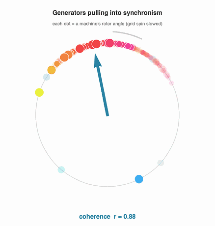
The generators pulling into synchronism. Each dot is a machine's rotor angle in the (slowed) spinning grid; the trails show the rotation. From a scattered start the machines swing in under their own inertia and lock into a co-rotating cluster – the coherence r climbing as they do. Shown in the lab frame so the synchronised grid keeps turning, rather than the rotating frame, which would freeze it into a still picture.
The same locking shown on the network: node colour is the voltage phase angle in the rotating frame. Scattered hues collapse to a single narrow band – the grid is synchronised.
6. Stability margin and the most-loaded line
6. Stability margin and the most-loaded line
As the coupling weakens, the phase differences across the lines grow to carry the same power through a stiffer-to-softer network. The line with the largest angle is the one closest to its static-stability limit of 90°; when that angle reaches 90°, the locked state is lost. Tracking the maximum line angle against K is therefore a direct read-out of the grid's distance to collapse.
Where does the power actually flow? Colouring and thickening each line by the active power it carries at the operating point shows the load-bearing arteries of the grid – and previews why one particular line will turn out to be critical.
7. N-1 contingency: which line failure desynchronises the grid?
7. N-1 contingency: which line failure desynchronises the grid?
First, the topology. Eleven of the 46 lines are radial – each is the only connection to a generator (the step-up transformers) or to a small sub-tree. Losing any of them instantly islands a machine: a trivial but real single point of failure.
The 11 topological single points of failure (red): lose one and a generator is cut adrift. These are bridges in the graph – no redistribution of flow can save them.
The interesting question is about the meshed core, where the graph stays connected and the flows merely redistribute. Here a clear winner emerges:
N-1 screen of the meshed lines. The outage of line 28–29 (red) raises the critical coupling from 0.17 to 0.34 – it more than doubles the coupling the grid needs to stay locked, far more than any other single line.
A second opinion: thermal limits and loadability
A second opinion: thermal limits and loadability
IEEE 39-bus line loadings at the operating point (blue low red high; width ∝ loading), with the worst thermal N-1 corridor 21–22 in red. Lines sit at 40–76% of their thermal rating.
Three legitimate definitions of "the critical line" now give three different answers for New England: the most-loaded line (first to overload as demand grows) is 16–19; the worst thermal N-1 (whose outage overloads another line, to 160%) is 21–22; and the weakest for synchronisability is 28–29. For the GB grid all three land in the southern peninsula (1–3, 2–4, 3–4) – the region is robustly critical even though the exact line depends on the criterion.
8. Watching the grid fall apart
8. Watching the grid fall apart
Identification by static fixed-point analysis is one thing; seeing the desynchronisation unfold is another. We stress the grid to a coupling K = 0.25 – still safely synchronised intact – start every machine from its locked state, and at t = 0 trip a single line. For a benign line the grid re-locks within a few cycles. For line 28–29 the generator cluster at bus 38 tears away and never recovers.
Node frequency deviations after the trip. Left: losing line 16–24, the swing damps out and the grid re-locks. Right: losing line 28–29, the bus-38 machines run away at their own frequency – a loss of synchronism that, on a real grid, trips protection and shed load.
The same event on the network, each bus coloured by phase. After 28–29 (red) trips, the colours drift apart instead of holding – the visual signature of a grid losing synchrony.
9. The energy transition: inertia, RoCoF and where the power comes from
9. The energy transition: inertia, RoCoF and where the power comes from
The same demand surge, three inertia levels. All settle at the same droop offset, but the low-inertia grid (red, high renewables) plunges to a much deeper nadir, much faster – the central frequency-stability worry of inverter-dominated grids.
Second, the transition moves where power is injected – from a few large thermal plants to many distributed resources. Because the critical line is set by the pattern of injections relative to the topology (Section 7), changing the generation mix can move the critical corridor entirely. The same machinery in this notebook – swap kgInjection for a renewable-heavy scenario and re-run kgContingency – becomes a screening tool for those questions.
10. The same machinery on the real National Grid
10. The same machinery on the real National Grid
The layout is the published geographic schematic: Scotland top-left, the Midlands and the huge generation hub at bus 16 in the centre, and the south-east of England – including the enormous London demand at bus 25 – bottom-right. Node area is the net power injection: generation-heavy buses (red) in the north and centre, the demand sinks (still red where they also generate) and the five pure load/junction buses (blue).
The reduced GB National Grid as a network of coupled oscillators. The diagonal silhouette is Britain; the radial "tail" at the bottom right is the south-east England peninsula (buses 1–4).
Every routine from the previous nine sections now works unchanged. The synchronisation transition:
The GB grid synchronises above K_c ≈ 0.19 and operates at K = 1 – a healthy five-fold margin, just like New England, and just as a real grid should.
And the N-1 contingency screen – the question that motivated the whole notebook – points to a clear answer for Britain:
GB N-1 screen. Two corridors stand out together: 3–4 and 2–4, the parallel pair that connects the south-east England peninsula (buses 1, 2, 3) to the rest of the grid. Losing either roughly doubles the coupling the grid needs.
The story is the same shape as New England's, on a different map. Buses 1, 2 and 3 form a generation-surplus pocket in the south-east; their only way out is the pair of corridors into bus 4. Lose one and the entire surplus squeezes through its twin, driving it to the stability limit. There are no purely radial single-points-of-failure here – the GB model is two-edge-connected (every double circuit merged into one corridor), so the vulnerability is genuinely a flow-redistribution effect, not a topological accident.
Power flows on the GB grid at K = 1 (line colour and width), with the critical southern gateway 3–4 in red.
As before, time-domain simulation confirms the static result. Stress the grid to K = 0.28, trip a single corridor, and watch the machine frequencies:
Left: losing a benign corridor, the GB grid re-locks. Right: losing 3–4, the south-east cluster pulls away to its own frequency – loss of synchronism.
The desynchronisation on the map of Britain: after corridor 3–4 (red) trips, the south-east peninsula's colours drift away from the rest of the country.
Finally, the two grids side by side. Both are operated at K = 1, comfortably above the critical coupling of their worst single-line outage – both are N-1 secure. But in each case it is one specific, identifiable line that sets the margin: 28–29 for New England, 3–4 for Great Britain.
Two real grids, the same method, the same conclusion: a single weakest link sets the synchronisation margin.
11. Checks against real grid data
11. Checks against real grid data
A model of the grid is only worth anything if it agrees with the real grid. The framework here makes three testable claims, and each can be checked against measured data from Great Britain's transmission system. The system operator (NESO) publishes the GB system frequency at one-second resolution; we use it directly.
Claim 1 – the grid sits in a phase-locked state at 50 Hz
Claim 1 – the grid sits in a phase-locked state at 50 Hz
Claim 2 – the inertial response is set by the swing equation
Claim 2 – the inertial response is set by the swing equation
Claim 3 – a single line outage really can desynchronise a grid
Claim 3 – a single line outage really can desynchronise a grid
The central result – that losing one line can split a synchronised grid – is not hypothetical. On 4 November 2006 a single planned line switching in northern Germany, mishandled, cascaded into a split of the entire Continental European synchronous area into three desynchronised islands within seconds, cutting power to more than 15 million households. That is precisely the loss-of-synchronism this notebook identifies line by line: the difference between a grid that re-locks after a disturbance and one that tears apart.
Taken together: the locked state is real (Claim 1), its inertial dynamics follow the swing equation we use (Claim 2), and line-outage desynchronisation is a documented failure mode (Claim 3). The model's added value is to say, for a given network, which line.
12. The real grid in real time
12. The real grid in real time
So far the GB injections came from a flat proportional dispatch – every generator scaled equally to meet demand. A real grid never looks like that: it runs a specific generation mix, made by specific power stations, in specific places. This section feeds the model nothing but real, openly-licensed data, downloaded live: where the power stations actually are, what they actually generated, and how the grid actually behaved – none of it redistributed here, all of it fetched by the cells below and cached locally.
Where the power really is
Where the power really is
It is tempting to spread each fuel across the network by a hand-drawn rule (wind to the north, solar to the south). That is a guess – and an easy one to get backwards. Instead we take the Global Power Plant Database (World Resources Institute, CC-BY, via the OSUKED Power Station Dictionary), with every GB station's location, fuel and capacity, and assign each plant to its nearest network bus. The geography is now measured, not assumed.
Every GB plant in the Global Power Plant Database, assigned to its nearest bus. Left: dominant fuel per bus (gas and nuclear dominate by capacity, so wind is not the headline colour). Right: installed capacity by latitude – wind's distribution sits modestly north of solar's (capacity-weighted mean 54.5°N vs 52.1°N), the geography that drives the B6 transfer. Capacities are the database's 2019 vintage (hence the surviving coal), so the geography is current even if a few plants have since retired.
Realistic dispatch: where the power flows
Realistic dispatch: where the power flows
Now take two real GB days – the windiest and the calmest day of January 2024 (live from the Carbon Intensity API), with real demand from Elexon BMRS – and drop each straight onto that real placement. Both synchronise at K = 1, but the flows are completely different.
Power flows on two real days under real placement. Left (windy, 57% wind): Scottish wind floods south toward English demand, so the north-south spine carries heavy transfer (dark, thick), and the most-loaded corridor (red) is up in Scotland. Right (calm, 15% wind): generation sits closer to load and the flows stay lighter. This is the real "wind in Scotland, demand in England" problem – and it now emerges from the data, rather than being drawn in by hand.
The B6 boundary: where it costs real money
The B6 boundary: where it costs real money
That north-south flow has a name and a price. The B6 boundary is the set of circuits along the Scotland-England border; NESO publishes its transfer limit and the cost of keeping flows within it. We sum the model's flow across the Scottish cut and compare it to the real limit, sweeping a whole month of real generation mixes.
Modelled ScotlandEngland transfer vs wind share, over a month of real half-hourly mixes (demand held fixed to isolate the wind effect), against the real B6 limit ≈ 4.6 GW (NESO year-ahead). Above ~30% wind the modelled transfer crosses the physical limit – which in reality is exactly when NESO must pay generators to not generate. GB-wide thermal+inertia constraint spend was £1.1 billion in 2023-24 (real NESO data, across all boundaries – B6 a major component). The windiest January day pushes the modelled transfer to ~7 GW, well past the limit.
A real half-hour, placed to the megawatt
A real half-hour, placed to the megawatt
We can go all the way to a single real settlement period. Elexon BMRS dataset B1610 reports the actual output of every GB Balancing Mechanism Unit; the Power Station Dictionary locates each unit. Nothing is synthetic – both the mix and its geography are measured.
A real metered half-hour (15 Jan 2024, 10:00). Every generating unit is placed at its actual station; 81% of GB output is located this way (the remainder is small embedded plant). Node colour = net injection, edge = |flow|. The model takes the real dispatch and synchronises it – no free parameters in the injection at all.
The margin across a whole year
The margin across a whole year
A full year of real GB mix through the model (demand held at the annual mean to isolate the mix). The margin stays comfortably positive at K = 1 all year, but it thins with wind share almost perfectly (r = −0.95), and the lowest-margin decile – the windiest, lowest-inertia hours – adds up to ~880 hours a year. This is the synchronisability cost of the transition, measured rather than assumed.
And is any of this an artefact of how we snapped plants to buses? We jitter the real per-bus placement (log-normal noise, renormalised) over many draws and recompute.
Robustness to placement uncertainty (60 draws). Left: the windy day stays the harder case in the large majority of draws. Right: the critical corridor stays a Scottish / B6 corridor across the draws. The vulnerable region – the Scotland-England transfer – is robust; the exact line moves with the assumptions.
Inertia: the real mix, the real frequency
Inertia: the real mix, the real frequency
The generation mix sets something else the model cares about: inertia. Synchronous machines (gas, nuclear, hydro, biomass) store rotational energy and resist frequency change; wind, solar and interconnectors – connected through power electronics – do not. So the synchronous share of the real mix is a direct proxy for system inertia, and Section 9 predicts that less inertia means a faster, more volatile frequency. We can test that on real data: for twelve GB days spanning calm and windy conditions, we pair the day's synchronous share against the volatility of the measured 1-second frequency.
Each point is one real GB day (n = 12, Jan & Aug 2024; r = −0.74). Both axes are measured data, downloaded live: lower synchronous inertia goes with larger frequency volatility. That is the inertia-RoCoF relationship the swing equation encodes (Section 9; RoCoF ∝ 1/inertia is essentially an identity), so this corroborates the model's premise on real data rather than being a model output. Let us make it one.
The swing model as a predictor. Left: measured RoCoF volatility on the 12 days against system inertia, with the model curve (one calibrated noise amplitude) through it. Right: model-predicted vs measured, r = 0.71, within ~10% on average. The inertia-RoCoF link is now a model output tested against measured data, not a correlation between two measurements.
Put together, Sections 10–12 take the same handful of equations from a textbook benchmark, to the real British grid, to the real British grid on a real day – and at each step the model keeps agreeing with what the grid actually does.
13. Does it scale? A 1354-bus European grid
13. Does it scale? A 1354-bus European grid
Everything so far ran on grids of a few dozen buses. The same code – one registry, one solver – runs unchanged on the 1354-bus PEGASE model of the European high-voltage transmission network (power-grid-lib / pglib-opf). We download it live, parse it from MATPOWER format, and register it like any other network.
The 1354-bus PEGASE European transmission network, laid out by a spring embedding (the case ships no coordinates; parallel circuits are merged into corridors). It synchronises at K = 1 with order parameter r = 0.98 and a healthy stability margin λ₂ = 0.34 – the same phase-locked picture as New England, two orders of magnitude larger. Red = net generation, blue = net demand.
Full N-1 – pricing every one of 1991 lines by a critical-coupling continuation – is hopeless at this size. So we screen: rank lines by flow, then measure the operating-point margin λ₂ after the outage for the most-loaded ones (one solve each, no continuation).
Scalable N-1 on the European grid. Of the 60 most-loaded corridors, 26 are islanding bridges – radial single-points-of-failure whose loss splits the grid. Among the meshed corridors, the bars rank the ones whose outage thins the margin most – the method that found New England's line 28–29, unchanged on a grid 35× larger.
14. Emergent phenomena on the continental grid
14. Emergent phenomena on the continental grid
A grid this size shows behaviour the textbook cases are simply too small to exhibit. Four examples, all on the live-downloaded PEGASE network, all from the same handful of equations.
Inter-area oscillation modes
Inter-area oscillation modes
Linearising the swing equation about the synchronised state, the slowest eigenmodes of the (inertia-weighted) network Laplacian are the low-frequency inter-area oscillations real interconnections exhibit. We compute the mode shapes – which regions swing against which.
The four slowest inter-area modes. Node colour is the signed mode shape – red and blue are the two halves that swing against each other; the slowest splits the continent into its two largest opposed blocks, the kind of low-frequency inter-area oscillation real interconnections exhibit. (Mode frequencies are in normalised model units set by the chosen inertias, so it is the mode shapes and their ordering that are meaningful, not an absolute match to Hz.)
A cascading blackout
A cascading blackout
The mechanism behind real continental blackouts (the 4 Nov 2006 UCTE split): one line trips, its power reroutes onto neighbours, some of those exceed their limit and trip too. We give every line a capacity = α × its initial flow, trip the busiest line, and let the overloads propagate.
Top: one trip (left) reroutes and overloads neighbours, which trip in turn (centre), cutting much of the grid from the synchronous core (right). Bottom: blackout size from a single trip against the line tolerance α (capacity = α × initial flow – a stylised proportional-capacity model, not real MVA ratings). It falls as lines gain headroom but non-monotonically: with little headroom one fault blacks out most of the continent, and the curve has a genuinely irregular tail – cascades are not simply tamed by more margin.
Decarbonisation stress test
Decarbonisation stress test
Replacing synchronous machines with inverter-based renewables removes rotational inertia. Inertia does not change the synchronised steady state, but it governs the transient: we lose the largest generator and watch the system rate-of-change-of-frequency as inertia is withdrawn.
As synchronous inertia is withdrawn, the post-fault system RoCoF rises steadily (left) – a continental-scale version of the GB inertia story of Section 12. RoCoF and inertia are in normalised model units, so the renewable share at which a protective limit is crossed is calibration-dependent (for the illustrative limit drawn, ~60–65%); the robust point is the monotonic rise, not a specific threshold. The map (right) shows which buses see the fastest local frequency swing.
Basin stability: a result that does not transfer
Basin stability: a result that does not transfer
A landmark study (Menck et al. 2014) found that a node's basin stability – the probability the grid returns to sync after a large random kick there – is lowest at radial dead ends. We tested that on the continental grid: perturb a node's phase and frequency hard, integrate the swing dynamics, and count how often the grid re-synchronises.
The honest result (40 hard (phase, frequency) kicks per node, 44 nodes, 95% CIs): the grid re-synchronises after almost every single-node kick – dead ends average 0.94 ± 0.04 versus 0.95 ± 0.02 for well-connected buses, a difference well within error. The dead-end fragility seen on small synthetic grids does not reproduce here: this real continental grid is uniformly resilient to localised shocks. A reminder that results from toy topologies do not automatically scale.
15. What we can and cannot claim
15. What we can and cannot claim
The coupling dial K and the inertia/damping values are normalised. K = 1 is the physical susceptance pattern; sweeping K is a clean way to probe stability margins, but it is a modelling device, not a literal control knob. The transient time axis is in normalised units, not seconds.
The GB generation is a proportional dispatch. The reduced GB model lists installed capacity per bus, not an instantaneous dispatch. We scale every generator by a common factor so total generation meets demand – a transparent, reproducible choice, but not a merit-order economic dispatch. A different dispatch (more wind in Scotland, say) shifts the injection pattern and can move the critical corridor; that is exactly the kind of question the kgInjection hook is meant to let you explore.
The real-data comparison is a calibrated check, not a blind fit. The Section 11 swing-equation overlays use GB-realistic but lumped parameters (one inertia constant, one demand-noise amplitude). They show the model captures the right physics – the RoCoF, the nadir depth, the fluctuation width – not that it predicts them from first principles. The real grid's governor action, automatic load shedding and market structure are real features the phase model deliberately omits.
The Section 12 placement is real, but the bus assignment is approximate. Generation mix, demand, per-unit metered output (BMRS B1610) and frequency are all real and measured; power-station locations come from the Global Power Plant Database. We assign each plant to the nearest reduced-network bus, using our own affine geo-referencing of the published GB schematic – so the latitude (north-south) structure that carries the wind-north / B6 story is faithful, while the exact bus a given plant lands on is approximate. The B6-transfer conclusion survives jittering that assignment (Section 12); the exact critical line moves with it, so it is the vulnerable region – the Scotland-England corridor – not the single line, that the result robustly identifies. The GPPD capacities are a 2019 vintage, so a few listed plants have since retired. The B6 cut itself (which buses count as "Scotland") is also taken from that affine fit's latitude, so the exact transfer figure carries the same indicative-geography uncertainty; it is the existence and direction of a large wind-driven north-south transfer, not the precise gigawatt value, that the result establishes.
The data is downloaded, not redistributed. Every third-party dataset in Sections 11-12 is fetched live by the notebook (kgFetch) from its official, openly-licensed source and cached locally; none of it is shipped inside this notebook. The figures shown are our own derived output. If a download endpoint is unavailable when you run it, the committed figures still display – only the recomputation needs the network.
16. References
16. References
G. Filatrella, A. H. Nielsen, N. F. Pedersen (2008). Analysis of a power grid using a Kuramoto-like model. Eur. Phys. J. B 61, 485–491.
A. E. Motter, S. A. Myers, M. Anghel, T. Nishikawa (2013). Spontaneous synchrony in power-grid networks. Nature Physics 9, 191–197.
D. Witthaut, M. Timme (2012). Braess's paradox in oscillator networks, desynchronization and power outage. New J. Phys. 14, 083036.
F. Dőrfler, M. Chertkov, F. Bullo (2013). Synchronization in complex oscillator networks and smart grids. PNAS 110, 2005–2010.
T. Athay, R. Podmore, S. Virmani (1979). A practical method for the direct analysis of transient stability. IEEE Trans. PAS-98, 573–584. (the IEEE 39-bus data)
R. D. Zimmerman, C. E. Murillo-Sánchez, R. J. Thomas (2011). MATPOWER. IEEE Trans. Power Syst. 26, 12–19. (case39 source)
M. Belivanis, K. R. W. Bell (2010). Coordination of phase-shifting transformers to improve transmission network utilisation. University of Strathclyde. (the reduced GB transmission model; data via the University of Edinburgh OptEnergy network collection)
NESO / National Grid ESO. Historic System Frequency Data (1-second resolution). NESO Data Portal. (real GB frequency used for validation)
National Grid ESO (2019). Technical Report on the events of 9 August 2019. (the GB disturbance reproduced in Section 11)
UCTE (2007). Final Report – System Disturbance on 4 November 2006. Union for the Coordination of Transmission of Electricity. (the Continental European split)
Carbon Intensity API – NESO & University of Oxford. GB generation mix by fuel type (CC BY 4.0). carbonintensity.org.uk (Section 12 dispatch)
Elexon. Balancing Mechanism Reporting Service (BMRS): demand outturn and dataset B1610 (Actual Generation Output per Generation Unit). data.elexon.co.uk. "Contains BMRS data © Elexon Limited copyright and database right 2026."
Global Power Plant Database v1.3.0 – World Resources Institute (CC BY 4.0); GB plant locations, fuels and capacities, via the OSUKED Power Station Dictionary (MIT). (Section 12 real plant placement)
NESO. Year-Ahead Constraint Limits (B6 – SCOTEX boundary) and Constraint Breakdown Costs and Volume. NESO Data Portal, Open Government Licence. (Section 12 B6 limit and constraint cost)
S. Babaeinejadsarookolaee et al. (2019). The Power Grid Library for Benchmarking AC Optimal Power Flow Algorithms (pglib-opf). arXiv:1908.02788. (the 1354-bus PEGASE case in Sections 13–14; C. Josz et al., the original PEGASE datasets)
P. J. Menck, J. Heitzig, J. Kurths, H. J. Schellnhuber (2014). How dead ends undermine power grid stability. Nature Communications 5, 3969. (basin stability, Section 14)
Y. Kuramoto (1975). Self-entrainment of a population of coupled non-linear oscillators. Lecture Notes in Physics 39, 420–422.
17. Reproduce it yourself
17. Reproduce it yourself
Everything here is reproducible from the attached package. The whole figure pipeline regenerates with one script:
# from the repository root (first run downloads the open data into data/cache/)
wolframscript -file wolfram/render_figures.wls # IEEE 39-bus figures + animations
wolframscript -file wolfram/render_uk_figures.wls # GB National Grid figures
wolframscript -file wolfram/validation.wls # validation vs real NESO frequency
wolframscript -file wolfram/render_placement.wls # real plant placement (GPPD)
wolframscript -file wolfram/render_realgrid.wls # real dispatch + inertia (live)
wolframscript -file wolfram/render_b6.wls # B6 boundary vs real limit + cost
wolframscript -file wolfram/render_bmrs.wls # a real metered half-hour (BMRS)
wolframscript -file wolfram/render_margincurve.wls # year-long margin duration curve
wolframscript -file wolfram/render_pegase.wls # the 1354-bus PEGASE European grid
wolframscript -file wolfram/render_modes.wls # inter-area oscillation modes
wolframscript -file wolfram/render_cascade.wls # cascading blackout + animation
wolframscript -file wolfram/render_decarbon.wls # decarbonisation / RoCoF stress test
wolframscript -file wolfram/render_basin.wls # basin stability map
wolframscript -file community/build_notebook.wls # rebuild this notebook
Or interactively, switch grids and screen the contingencies of either network with the same one-liner:
Built in Wolfram Language. The companion package kuramoto_powergrid_helpers.wl is attached; the full repository (data, scripts, figures) accompanies this post.
CITE THIS NOTEBOOK
CITE THIS NOTEBOOK
Power-grid stability via the Kuramoto model on a real transmission network
by Marco Thiel
Wolfram Community, STAFF PICKS, June 22, 2026
https://community.wolfram.com/groups/-/m/t/3737769
by Marco Thiel
Wolfram Community, STAFF PICKS, June 22, 2026
https://community.wolfram.com/groups/-/m/t/3737769