Thermophysical Properties of Ethane,1,1-difluoro (R152a) from: https://webbook.nist.gov/cgi/fluid.cgi?ID=C75376&Action=Page
saturation properties - pressure increment = 0.1 bar
{Temperature (C), Pressure (bar), liq. Enthalpy (kJ/kg), liq. Entropy (J/g*K), vap. Enthalpy (kJ/kg), vap. Entropy (J/g*K)}
{Temperature (C), Pressure (bar), liq. Enthalpy (kJ/kg), liq. Entropy (J/g*K), vap. Enthalpy (kJ/kg), vap. Entropy (J/g*K)}
datasat=;
In[]:=
tblhl=Table[{datasat[[i]][[2]],datasat[[i]][[3]]},{i,1,Length[datasat]}];tblsl=Table[{datasat[[i]][[2]],datasat[[i]][[4]]},{i,1,Length[datasat]}];
In[]:=
fhl=Interpolation[tblhl];fsl=Interpolation[tblsl];
In[]:=
tblhv=Table[{datasat[[i]][[2]],datasat[[i]][[5]]},{i,1,Length[datasat]}];tblsv=Table[{datasat[[i]][[2]],datasat[[i]][[6]]},{i,1,Length[datasat]}];
In[]:=
fhv=Interpolation[tblhv];fsv=Interpolation[tblsv];
In[]:=
tblpt=Table[{datasat[[i]][[2]],datasat[[i]][[1]]},{i,1,Length[datasat]}];
In[]:=
fpt=Interpolation[tblpt];
isobaric properties - pressure = 10.14 bar
{Temperature (C), Pressure (bar), Enthalpy (kJ/kg), Entropy (J/g*K), State)}
{Temperature (C), Pressure (bar), Enthalpy (kJ/kg), Entropy (J/g*K), State)}
dataisobaric=;
In[]:=
pos=Position[dataisobaric,44.14]
Out[]=
{{283,1},{284,1}}
In[]:=
tblhsv=Table[{dataisobaric[[i]][[1]],dataisobaric[[i]][[3]]},{i,284,Length[dataisobaric]}];tblssv=Table[{dataisobaric[[i]][[1]],dataisobaric[[i]][[4]]},{i,284,Length[dataisobaric]}];
In[]:=
fhsv=Interpolation[tblhsv];fssv=Interpolation[tblssv];
Problem statement (reproduced from Ref. 1)Set-up of the refrigeration cycle with turbo-compression is depicted below:This set-up is composed of 2 cycles: 1- motor cycle with boiler, condenser, pump and turbine2- refrigeration cycle with evaporator, throttling valve, compressor, condenserASSUMPTIONS:The cycle is ideal. The energy provided by the turbine solely to drive the compressor (m4dot (h4 - h3) = - m10dot (h10 - h9)).Transformation in the throttling valve is an isenthalpic process (h7=h8). No sub-cooling and/or superheating in the condenser and the evaporator stages (T8=T9 et T5=T6).The mixer is ideal (P4=P10=P5). Steady-state is assumed. We neglect the variations in kinetic and potential energy.References:[1] D. Ronze, Coordonnateur, Introduction au génie des procédés: Applications et développements, Tec & Doc, Paris, Lavosier, 2013.
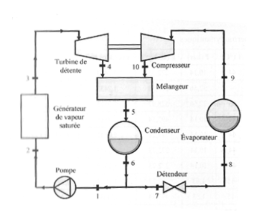
GIVEN: States of points: 3, 9, and 6 are Saturated Vapor, Saturated Liquid And Saturated VaporP3 = 32.56 bar ; P9 = 1.53 bar ; P6 = 10.14 bar. Average specific volume between points 1 and 2 is equal to 0.00118 m3/kg
point | T °C | P bar | h kJ/kg | s kJ/kg*K | state |
3 | 96.2156 | 32.56 | 539.231 | 1.98351 | sat. vap. |
6 | 44.1404 | 10.14 | 279.199 | 1.26558 | sat. liq. |
9 | -14.2949 | 1.53 | 497.079 | 2.15058 | sat. vap. |
In[]:=
P3=32.56;P9=1.53;P6=10.14;
In[]:=
POINT3={fpt[P3],P3,fhv[P3],fsv[P3]}
Out[]=
{96.2156,32.56,539.231,1.98351}
In[]:=
POINT6={fpt[P6],P6,fhl[P6],fsl[P6]}
Out[]=
{44.1404,10.14,279.199,1.26558}
In[]:=
POINT9={fpt[P9],P9,fhv[P9],fsv[P9]}
Out[]=
{-14.2949,1.53,497.079,2.15058}
In[]:=
{T9,P9,h9,s9}={fpt[P9],P9,fhv[P9],fsv[P9]}
Out[]=
{-14.2949,1.53,497.079,2.15058}
In[]:=
{T6,P6,h6,s6}={fpt[P6],P6,fhl[P6],fsl[P6]}
Out[]=
{44.1404,10.14,279.199,1.26558}
In[]:=
{T3,P3,h3,s3}={fpt[P3],P3,fhv[P3],fsv[P3]}
Out[]=
{96.2156,32.56,539.231,1.98351}
Let us determine the unknown variables for points {1, 2, 4, 5, 7, 8, 10} of the Table below:
point | T °C | P bar | h kJ/kg | s kJ/kg*K | state |
1 | T1 | P1 | h1 | s1 | sat. liq. |
2 | -- | P2 | h2 | s2 | compressed lid. |
3 | 96.2156 | 32.56 | 539.231 | 1.98351 | sat. vap. |
4 | T4 | P4 | h4 | s4 | quality4 |
5 | T5 | P5 | h5 | s5 | quality5 |
6 | 44.1404 | 10.14 | 279.199 | 1.26558 | sat. liq. |
7 | T7 | P7 | h7 | s7 | sat. liq. |
8 | T8 | P8 | h8 | s8 | quality8 |
9 | -14.2949 | 1.53 | 497.079 | 2.15058 | sat. vap. |
10 | T10 | P10 | h10 | s10 | super heated vap. |
In[]:=
P2=P3;P8=P9;P5=P6;
In[]:=
P1=P6;P7=P6;
In[]:=
P4=P5;P10=P5;
In[]:=
s4=s3;
In[]:=
s10=s9;
In[]:=
T1=T6;T7=T6;
In[]:=
T8=T9;
In[]:=
T5=T6;
In[]:=
T4=T5;T10=.
In[]:=
h7=h6;h8=h7;
In[]:=
T10=x/.FindRoot[fssv[x]==s10,{x,60}]
Out[]=
64.1134
In[]:=
h10=fhsv[T10]
Out[]=
560.833
In[]:=
(*slsat@P4<s4<svsat@P4point4isinthetwo-phaseregion*)
In[]:=
s4
Out[]=
1.98351
In[]:=
s4v=fsv[P4]
Out[]=
2.06645
Final Results
Efficiency is 42.377 %