A Galton board is a simple device: drop a ball through rows of pegs and it bounces left or right at each one, landing in a slot at the bottom. Do this thousands of times and the slots fill up in a bell curve, the famous normal distribution. The outcome is predictable in aggregate even though each individual bounce is random.
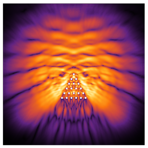
Now imagine the ball is replaced by a quantum particle. It no longer takes one path, it travels all paths at once as a wave, splitting and recombining at every peg. The different paths interfere with each other, like ripples on water, and the final distribution is nothing like a bell curve. This is the quantum Galton board.
This notebook simulates exactly that. A quantum wavepacket is launched downward through a triangular array of five rows of hard-wall obstacles and the full evolution of its probability density is computed by numerically solving the time-dependent Schrödinger equation. The result is rendered as both a static image and an exported animation, making the interference structure directly visible.
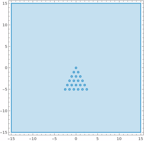
Creating the classical Galton geometry with 21 pegs. Each row r contains r+1 pegs horizontally spaced by 1 unit. Disk radius is δr = .2
n=5;δr=.2;pts=Flatten[Table[{k-r/2,-r},{r,0,n},{k,0,r}],1];
Defining the simulation domain Ω as a 30×30 bounding box with 21 circular disks.
In[]:=
s=15;Ω=RegionDifference[Rectangle[{-s,-s},{s,s}],RegionUnion[Disk[#,δr]&/@pts]]
Out[]=

In[]:=
reg=RegionPlot[Ω]
Out[]=
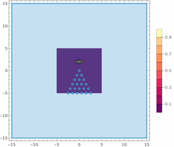
Initial wavepacket positioned above the top peg row
ic=Exp[-(y-2)^2/.1-I10y]Exp[-(x^2/(4δr)^2)];ShowContourPlotAbs[ic],{x,y}∈Rectangle[{-5,-5},{5,5}],,reg
Out[]=
Construct the 2D time-dependent Schrödinger operator iℏ+ with , .
H
∂
t
2
2m
2
∇
ℏ=1
m=1
In[]:=
ℋ=SchrodingerPDEComponent[{Ψ[t,x,y],t,{x,y}},<|"ReducedPlanckConstant"->1|>]
Out[]=
∇
{x,y}
1
2
1
2
∇
{x,y}
(1,0,0)
Ψ
In[]:=
Needs["NDSolve`FEM`"]
Mesh generation
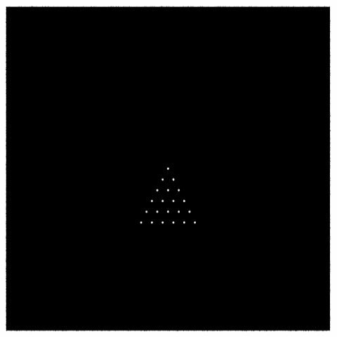
mesh=ToElementMesh[Ω,"MaxCellMeasure"->0.01,AccuracyGoal->4]
Out[]=
ElementMesh[{{-15.,15.},{-15.,15.}},{TriangleElement[<155522>]}]
In[]:=
mesh["Wireframe"]
Out[]=
In[]:=
mesh["Coordinates"]//Length
Out[]=
314088
Simulation end time
In[]:=
tEnd=0.75;
Solution of time-dependent Schrödinger equation
In[]:=
AbsoluteTiming[MaxMemoryUsed[Monitor[solution=NDSolveValue[{ℋ==0,Ψ[0,x,y]==ic,DirichletCondition[Ψ[t,x,y]==0,True]},Ψ,{t,0,tEnd},{x,y}∈mesh,EvaluationMonitor:>(monitor=Row[{"t = ",CForm[t]}])];,monitor]]/1024.^2]
Out[]=
{1246.32,2295.88}
Export the solution so that you don’t have to re-run the above code next time you return to this simulation.
Export["~/solution.mx",solution]
Plot the final probability density
DensityPlotAbs[solution[tEnd,x,y]],{x,y}∈mesh,ColorFunction->(ColorData["SunsetColors"][Sqrt[#]]&),
Out[]=
Generating the frames during the full period of the simulation Δt = 0.01 → 0.76
frames=TablePrintTemporary["t: ",t];DensityPlotAbs[solution[t,x,y]],{x,y}∈mesh,,{t,0,tEnd,0.01};
Show the generated frames as an animation
In[]:=
ListAnimate[frames]
Out[]=
CITE THIS NOTEBOOK
CITE THIS NOTEBOOK
The quantum Galton board: FEM simulation of 2D wavepacket interference
by Mohammad Bahrami
Wolfram Community, STAFF PICKS, April 15, 2026
https://community.wolfram.com/groups/-/m/t/3688834
by Mohammad Bahrami
Wolfram Community, STAFF PICKS, April 15, 2026
https://community.wolfram.com/groups/-/m/t/3688834