In this work, I demonstrate modeling of the cart-pole system using both component-oriented modeling and ‘manual’ equation-based modeling. I compare the speed of and outputs from the two types of models, and I experiment with performance of different compiler options for SystemModeler on Windows 10 (Xeon E3-1230v3 3.30GHz CPU). I hope this project can be useful to anyone willing to start learning SystemModeler.
Background
Background
The cart pole system is a simple mechanical system involving a pole which is free to rotate about a pivot centered on a cart (which is often controlled by some input force). This system is often used as a simple reinforcement learning task and is featured in the popular OpenAI Gym environment. SystemModeler is a nice environment for modeling physically-based dynamical systems, and it could have a large degree of applicability to the future of increased use of tools like ‘digital twins’ for process monitoring, simulation, control, and RL agent training.
Also, Wang Zhang of WRI gave an interesting talk on the possibilities of using SystemModeler for RL where he shows his own cart-pole system model: https://www.wolfram.com/broadcast/video.php?c=104&p=2&v=2139
Also, Wang Zhang of WRI gave an interesting talk on the possibilities of using SystemModeler for RL where he shows his own cart-pole system model: https://www.wolfram.com/broadcast/video.php?c=104&p=2&v=2139
Modeling Cart-Pole systems with SystemModeler
Modeling Cart-Pole systems with SystemModeler
We begin by creating a basic CartPole model using SystemModeler. I begin with a fast component-oriented modeling approach to build a cart-pole system out of Modelica standard library component blocks:
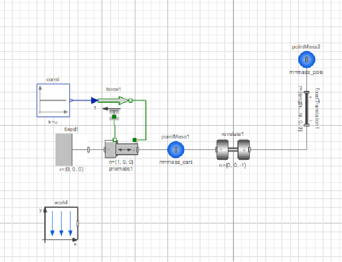
model CartPole "A simple cart-pole system"
import Modelica.Constants.pi;
parameter Real g = 9.81 "gravitational constant";
parameter Real mass_cart = 1 "kg";
parameter Real mass_pole = 1 "kg, equivalent mass at end of 'massless' pole";
parameter Real length_pole = 2 "m";
parameter Real theta0 = -pi / 2 "starting angle of pole";
parameter Real u = 1 "N";
Modelica.Mechanics.MultiBody.Joints.Prismatic prismatic1(animation = false, useAxisFlange = true, s.start = 0) annotation(Placement(visible = true, transformation(origin = {-68.273, -15}, extent = {{-10, -10}, {10, 10}}, rotation = 0)));
inner Modelica.Mechanics.MultiBody.World world(enableAnimation = true) annotation(Placement(visible = true, transformation(origin = {-105, -60}, extent = {{-10, -10}, {10, 10}}, rotation = 0)));
Modelica.Mechanics.MultiBody.Parts.FixedTranslation fixedTranslation1(r = {length_pole, 0, 0}) annotation(Placement(visible = true, transformation(origin = {45, 10}, extent = {{-10, -10}, {10, 10}}, rotation = -90)));
Modelica.Mechanics.MultiBody.Joints.Revolute revolute1(phi.start = theta0 + 3.1415926535, n = {0, 0, -1}, phi.fixed = true, useAxisFlange = false) annotation(Placement(visible = true, transformation(origin = {0, -15}, extent = {{-10, -10}, {10, 10}}, rotation = -180)));
Modelica.Mechanics.MultiBody.Parts.PointMass pointMass2(m = mass_pole) annotation(Placement(visible = true, transformation(origin = {45, 40}, extent = {{-10, -10}, {10, 10}}, rotation = 0)));
Modelica.Mechanics.MultiBody.Parts.Fixed fixed1 annotation(Placement(visible = true, transformation(origin = {-98.489, -15}, extent = {{-10, -10}, {10, 10}}, rotation = 0)));
Modelica.Blocks.Sources.Constant const(k = u) annotation(Placement(visible = true, transformation(origin = {-110, 15}, extent = {{-10, -10}, {10, 10}}, rotation = 0)));
Modelica.Mechanics.Translational.Sources.Force force1(useSupport = true) annotation(Placement(visible = true, transformation(origin = {-72.699, 15}, extent = {{-10, -10}, {10, 10}}, rotation = 0)));
Modelica.Mechanics.MultiBody.Examples.Elementary.PointGravityWithPointMasses2.PointMass pointMass1(m = mass_cart, r_0.start = {0, 0, 0}, each r_0.fixed = true) annotation(Placement(visible = true, transformation(origin = {-35, -15}, extent = {{-10, -10}, {10, 10}}, rotation = 0)));
public
Real angle "Angle of the cart's pole";
Real position "Cart position";
Real velocity "velocity of the cart";
equation
connect(fixedTranslation1.frame_a, pointMass2.frame_a) annotation(Line(visible = true, origin = {45, 30}, points = {{0, -10}, {0, 10}}, color = {95, 95, 95}));
connect(fixed1.frame_b, prismatic1.frame_a) annotation(Line(visible = true, origin = {-83.381, -15}, points = {{-5.108, 0}, {5.108, 0}}, color = {95, 95, 95}));
connect(force1.flange, prismatic1.axis) annotation(Line(visible = true, origin = {-57.38, 3}, points = {{-5.319, 12}, {4.106, 12}, {4.106, -12}, {-2.894, -12}}, color = {0, 127, 0}));
connect(force1.support, prismatic1.support) annotation(Line(visible = true, origin = {-72.486, -1}, points = {{-0.213, 6}, {-0.213, 1}, {0.213, 1}, {0.213, -8}}, color = {0, 127, 0}));
connect(const.y, force1.f) annotation(Line(visible = true, origin = {-91.849, 15}, points = {{-7.151, -0}, {7.151, 0}}, color = {1, 37, 163}));
connect(prismatic1.frame_b, pointMass1.frame_a) annotation(Line(visible = true, origin = {-46.637, -15}, points = {{-11.636, 0}, {11.637, 0}}, color = {95, 95, 95}));
connect(pointMass1.frame_a, revolute1.frame_b) annotation(Line(visible = true, origin = {-20, -15}, points = {{-15, 0}, {10, 0}}, color = {95, 95, 95}));
connect(revolute1.frame_a, fixedTranslation1.frame_b) annotation(Line(visible = true, origin = {33.333, -10}, points = {{-23.333, -5}, {11.667, -5}, {11.667, 10}}, color = {95, 95, 95}));
position = pointMass1.r_0[1];
velocity = pointMass1.v_0[1];
angle = (revolute1.phi-pi);
annotation(Diagram(coordinateSystem(extent = {{-150, -90}, {150, 90}}, preserveAspectRatio = true, initialScale = 0.1, grid = {5, 5})), Icon(coordinateSystem(extent = {{-100, -100}, {100, 100}}, preserveAspectRatio = true, initialScale = 0.1, grid = {10, 10}), graphics = {Rectangle(visible = true, lineColor = {128, 0, 0}, fillColor = {255, 0, 0}, pattern = LinePattern.None, fillPattern = FillPattern.Sphere, extent = {{-100, -100}, {100, 100}}, radius = 25), Polygon(visible = true, rotation = -45, lineColor = {255, 255, 255}, fillColor = {255, 255, 255}, fillPattern = FillPattern.Solid, points = {{-90, -15}, {-90, -15}, {-15, 50}, {-15, 50}, {-15, 80}, {-15, 95}, {-5, 115}, {5, 115}, {15, 95}, {15, 80}, {15, 50}, {15, 50}, {90, -15}, {90, -15}, {90, -30}, {90, -30}, {45, -5}, {45, -5}, {15, 5}, {15, 5}, {15, -30}, {10, -50}, {10, -50}, {35, -75}, {35, -75}, {35, -85}, {35, -85}, {5, -75}, {5, -75}, {5, -80}, {0, -85}, {-5, -80}, {-5, -75}, {-5, -75}, {-35, -85}, {-35, -85}, {-35, -75}, {-35, -75}, {-10, -50}, {-10, -50}, {-15, -30}, {-15, 5}, {-15, 5}, {-45, -5}, {-45, -5}, {-90, -30}, {-90, -30}}, smooth = Smooth.Bezier)}));
end CartPole;
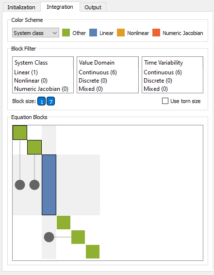
According to SystemModeler, our system contains 36 equations with 25 of them being trivial.
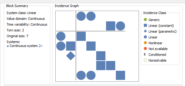
The incidence graph for the largest block shows it consists of 7 equations:
For comparison, I build a simple “CartPoleFast” Modelica class that has all equations for the dynamics of our CartPole system. We can use our knowledge of the system to build a more minimal representative coordinate frame involving only the position of the cart and the angle of the pole. Here is the resulting Modelica class:
model CartPoleFast "a fast, pure modelica cart-pole model"
// imports
import Modelica.Constants.pi;
// paramters
parameter Real mc = 1 "kg, mass of the cart";
parameter Real mp = 1 "kg, mass of point-mass-equivalent of pole";
parameter Real rp = 1 "m, length of pole";
parameter Real u = 1 "N, input force to the system";
parameter Real g = 9.81 "gravitational constant";
//initial state
parameter Real x_start = 0;
parameter Real v_start = 0;
parameter Real th_start = -pi / 2 "starting theta angle of pole";
parameter Real w_start = 0 "starting angular velocity of pole";
public
// simulation variables
Real x "cart linear position";
Real v "cart linear velocity";
Real th "pole angle, internal coordinate frame";
Real w "pole angular velocity";
Real angle;
protected
//Real rcy "reaction force of cart in y direction";
initial equation
x = x_start;
v = v_start;
th = -th_start + pi/2;
w = w_start;
algorithm
angle := -(th - pi/2);
equation
// derivative relationships
der(x) = v;
der(th) = w;
// Florian 2005, https://www.researchgate.net/publication/228808375_Correct_equations_for_the_dynamics_of_the_cart-pole_system
der(w) * rp * (1 - (mp * cos(th)^2) / (mp+mc)) = g * sin(th) + cos(th) * (-u - mp*rp*w^2*sin(th)) / (mc + mp);
der(v) * (mc + mp) = u + mp * rp * (w^2*sin(th) - der(w)*cos(th));
annotation(Icon(coordinateSystem(extent = {{-100, -100}, {100, 100}}, preserveAspectRatio = true, initialScale = 0.1, grid = {10, 10}), graphics = {Rectangle(visible = true, fillColor = {0, 0, 255}, fillPattern = FillPattern.Solid, extent = {{-43.642, -27.005}, {43.642, 27.005}}), Line(visible = true, origin = {0, 30}, points = {{0, 30}, {0, -30}}, thickness = 5), Ellipse(visible = true, origin = {0, 67.47}, fillColor = {255, 0, 0}, fillPattern = FillPattern.Solid, extent = {{-15, -15}, {15, 15}}), Line(visible = true, origin = {-76.802, 20}, points = {{-21.083, 0}, {21.083, 0}}), Line(visible = true, origin = {-66.486, 7.992}, points = {{-10, 0}, {10, 0}}), Line(visible = true, origin = {-76.182, -7.53}, points = {{-18.19, 0}, {18.19, 0}}), Line(visible = true, origin = {-66.644, -16.063}, points = {{-9.154, 0}, {9.154, 0}})}), experiment(StopTime = 10.0));
end CartPoleFast;
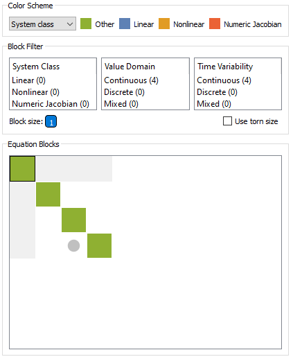
This model contains 5 equations (3 trivial). The model built by SystemModeler only consists of 4 single-equation blocks:
Both the component-oriented CartPole model and the hand-written CartPoleFast model agree numerically, a fact I found extremely impressive considering the CartPoleFast model took me several days of playing with physics equations before I gave up and used someone else’s dynamics equations while I was able to complete the CartPole component-oriented model in a matter of minutes. Additionally, CartPoleFast is only offers a 7.5% performance increase over the component-oriented model despite the component-oriented model containing many more equations. This could be because both programs are small relative to the size of l-1 cache on my computer.With animation disabled, the CartPole component-based model takes an average of 4 seconds to simulate 1000 seconds, requiring 149571 function evaluations with DASSL at 1e-6 tolerance.The CartPoleFast hand-written dynamics model (has no animation) takes an average of 3.7 seconds to simulate 1000 seconds, requiring 150618 function evaluations with DASSL at 1e-6 tolerance. With animation enabled, the CartPole component-based model takes an average of 6.62 seconds with the same solver settings.Here is a comparison of the output of the two models with the same starting conditions (0.1N input force, starting with the arm at 0 degrees (straight out), 1kg cart and pole point-masses, 2m-long pole):
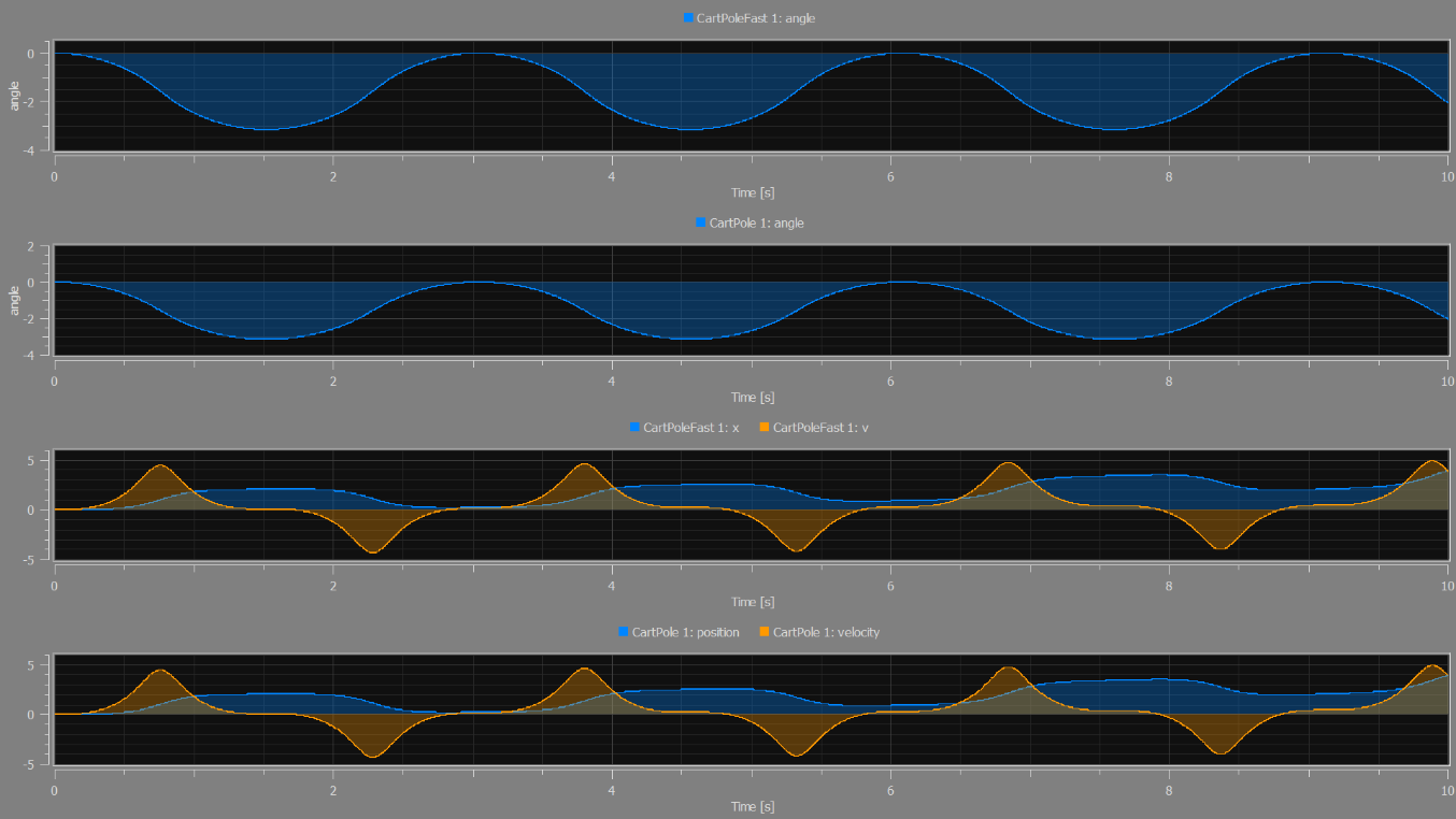
These results validate our component-oriented model . It seems that component-oriented modeling significantly speeds up my modeling workflow while minimally impacting model performance. Furthermore, the component-oriented CartPole model is significantly easier to extend to add friction forces, drag, and other items to improve model fidelity.
Compiler Optimizations Exploration
Compiler Optimizations Exploration
We will now experiment with multiple different compilers. We begin with the Intel compiler environment downloaded through Intel oneAPI:
The CartPoleFast model is probably too small to use as any kind of compiler benchmark.
I will instead switch to the CartPole (component-oriented) model with animation enabled for further compiler testing. This model becomes much larger when animation is enabled, so hopefully different compiler options will be exaggerated.
Using “C:\Program Files (x86)\Intel\oneAPI\setvars.bat” environment and compiler flags “/MT /EHa /FS /O2 /p:Configuration=”Release” /fp:fast”:
Build finished at 20:49:47 (took 02:08). Integration takes an average of 5.00 s/1000s (lowest 4.8s/1000s).
Using default Visual Studio Build Tools 2019 64-bit, “C:\Program Files (x86)\Microsoft Visual Studio\2019\BuildTools\Common7\Tools\VsDevCmd.bat” default settings , Build finished at 20:59:12 (took 00:10), integration takes an average of 5.9s (lowest 5.8s).
Using “C:\Program Files (x86)\Microsoft Visual Studio\2019\BuildTools\Common7\Tools\VsDevCmd.bat” with flags “/MT /EHa /FS /O2”, build finished at 21:05:18 (took 01:21), integration takes an average of 5.00 s (lowest 4.9s).
CartPole (component-oriented) model without animation:
Using “C:\Program Files (x86)\Microsoft Visual Studio\2019\BuildTools\Common7\Tools\VsDevCmd.bat” with flags “/MT /EHa /FS /O2”, build took 00:03, integration takes an average of 3.75 s (lowest 3.70s).
Using “C:\Program Files (x86)\Microsoft Visual Studio\2019\BuildTools\Common7\Tools\VsDevCmd.bat” with flags “/MT /EHa /FS ”, build took 00:03, integration takes an average of 3.75 s (lowest 3.64s).
For larger models, the /02 compiler option can result in around a 15% speedup at the cost of a 7x increase in compilation time. This might be worth noting when planning on releasing compiled models in FMUs for reinforcement learning. For smaller models there is no apparent speedup associated with using the /O2 compiler flag.
Switching to the Intel compiler environment is not enough to improve performance significantly for our simple architectures. I do not know if such a switch actually changes the compiler executable and enables Intel optimizations. Perhaps most compilers are near optimal for this class of program and changing compilers will generally result in little speedup, or perhaps this specific system is too small to exploit any parallelism and there would be a more significant speedup from different compilers when using more complex or parallelizable models.