Recovering Curve Length from Data: An Arc-Length Approach
Authors: Housam Binous
Recovering Curve Length from Data: An Arc-Length Approach
Authors: Housam Binous
Authors: Housam Binous
We presents a numerical method for estimating the length of a planar curve from discrete data points. The approach combines interpolation with a differential formulation that enforces arc-length parametrization, allowing the curve length to be computed directly from the solution of a differential algebraic system of equations (DAEs).Given a set of data points , an interpolating function is first constructed. Instead of evaluating the classical arc-length integral,which can be sensitive to noise and numerical differentiation, we reformulate the problem dynamically.We introduce a parametrization such that the parameter represents arc length. This is enforced through the constraint,together with the geometric condition:.This leads to a coupled system of differential algebraic equations, which is solved numerically using NDSolve. Once the system is solved, the curve length is obtained directly from the parameter s, eliminating the need for post-processing integration.The method is first validated on a semicircle of radius a=3, where the exact arc length is known to be L = aπ = 9.4247. Using interpolated data points, the computed length closely approximates the exact value, with small discrepancies arising from interpolation error, finite sampling, and initial tangent approximation.The approach is then applied to synthetic noisy data. In this case, interpolation (linear or higher-order) defines the curve geometry, and the DAE-based arc-length parametrization provides a robust way to estimate length even when the data is irregular or noisy.This method offers several advantages:It avoids direct differentiation of noisy data.It provides a geometrically consistent parametrization.It is flexible and applicable to arbitrary datasets.However, accuracy depends on interpolation quality, sampling density, and appropriate initial conditions for the differential system.In summary, the notebook demonstrates that arc-length computation can be effectively reformulated as a dynamical problem, providing a powerful alternative to classical integral-based methods for data-driven curves.
(xi,yi)
y=f(x)
L=∫
1+
x2
(f'(x))
(x(s),y(s))
s
x'+y'=1
2
(s)
2
(s)
y(s)=f(x(s))
Test problem: a section of a curve with known length (Semicircle case)
In[]:=
a=3.;
In[]:=
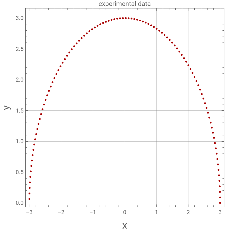
data=Table[{aCos[t],aSin[t]},{t,0,Pi,0.03}];
In[]:=
p1=ListPlot[data,PlotLabel->"experimental data",AspectRatio->1,Frame->True,GridLines->Automatic,PlotStyle->{Thick,Darker@Red},AspectRatio->1,FrameLabel->{Style["x",16],Style["y",16]}]
Out[]=
In[]:=
L_exact=aPi
Out[]=
9.42478
Method based on arc-length continuation and data interpolation
In[]:=
Clear[x,y]
In[]:=
f=Interpolation[data,InterpolationOrder->3]
Out[]=
InterpolatingFunction


In[]:=
eq1=y[s]==f[x[s]](*equationofanellipse*)
Out[]=
y[s]InterpolatingFunction[x[s]]
In[]:=
eq2=x'[s]^2+y'[s]^2==1(*auxiliaryequation*)
Out[]=
2
′
x
2
′
y
In[]:=
SOL=Quiet@First@NDSolve[{eq1,eq2,x[0]==0,y[0]==a,x'[0]==-0.1,y'[0]==0.1},{x,y},{s,-40,40},AccuracyGoal->12]
Out[]=
xInterpolatingFunction,yInterpolatingFunction


In[]:=
FindRoot[(y[s]/.SOL)==0,{s,7}]
Out[]=
{s4.71242}
In[]:=
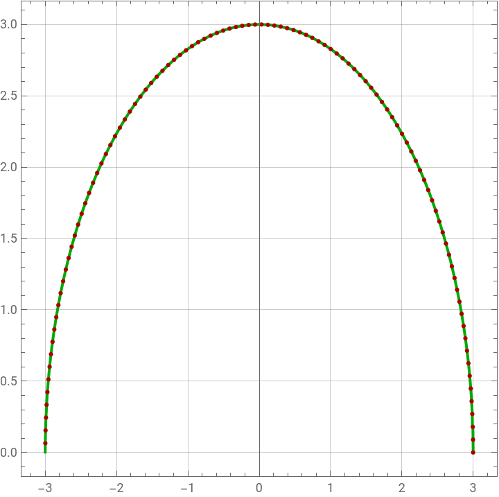
p2=ParametricPlot[{x[s],y[s]}/.SOL,{s,-4.71,4.71},Frame->True,PlotRange->All,GridLines->Automatic,PlotStyle->{Thick,Darker@Green},ImageSize->Medium,AspectRatio->1,PlotPoints->1000];
In[]:=
L_fromdata=2s/.FindRoot[(x[s]/.SOL)==-a,{s,5}]
Out[]=
9.34402
In[]:=
Show[p2,p1]
Out[]=
Method based on arc - length continuation applied to synthetic experimental data (case with unknown length of the arc of the curve)
In[]:=
SeedRandom[2];
In[]:=
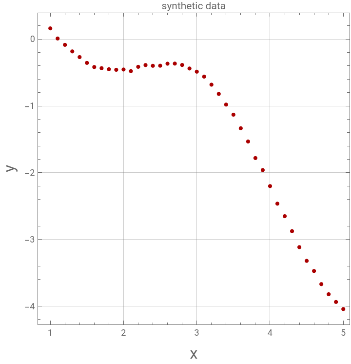
data=Table[{i,-i^2/6+Cos[i]^2+0.05RandomReal[]},{i,1,5,0.1}]
Out[]=
{{1.,0.161372},{1.1,0.00955521},{1.2,-0.0851617},{1.3,-0.183332},{1.4,-0.268619},{1.5,-0.355299},{1.6,-0.417556},{1.7,-0.435003},{1.8,-0.450668},{1.9,-0.458594},{2.,-0.45456},{2.1,-0.47895},{2.2,-0.414195},{2.3,-0.38812},{2.4,-0.39873},{2.5,-0.397585},{2.6,-0.36734},{2.7,-0.365966},{2.8,-0.386773},{2.9,-0.439413},{3.,-0.486666},{3.1,-0.561202},{3.2,-0.681622},{3.3,-0.819973},{3.4,-0.980035},{3.5,-1.13104},{3.6,-1.33485},{3.7,-1.53302},{3.8,-1.78062},{3.9,-1.9609},{4.,-2.20085},{4.1,-2.46387},{4.2,-2.65141},{4.3,-2.87609},{4.4,-3.11557},{4.5,-3.32034},{4.6,-3.47214},{4.7,-3.66899},{4.8,-3.82041},{4.9,-3.93605},{5.,-4.04224}}
In[]:=
p1=ListPlot[data,PlotLabel->"synthetic data",AspectRatio->1,Frame->True,GridLines->Automatic,PlotStyle->{Thick,Darker@Red},AspectRatio->1,FrameLabel->{Style["x",16],Style["y",16]}]
Out[]=