This notebook series is designed to introduce selected dynamic economic models to both advanced undergraduate and graduate students. Economists have relied on a series of economic models to better understand the otherwise highly complex causal relationship among many economic variables. Dynamic economic models set up by systems of either difference or differential equations are particularly useful in tracing the change in the quantity of unknown economic variables (e.g., the capital stock, demand for labor, aggregate output, etc.) and their interactions over time.
This notebook series aims to help students better understand the depth, usefulness, and limitations of major existing micro and macroeconomic models by demonstrating how we can use Wolfram Mathematica to replicate and reconstruct the core ideas and find dynamic solution of the model.
The model introduced in this notebook series include, among others, (1) the cobweb model of the quantity and price adjustment, (2) Keynes’s aggregate demand model, (3) Hicks’s ISLM model, (4) Samuelson’s investment accelerator model, (5) Kalecki’s investment delay model, (6) the predator-prey interaction model, (7) the epidemic model, (8) Ricardo’s three dimensional business cycle model, (9) Marx-Goodwin business cycle and growth model, (10) Smith’s and Ricardo’s growth model, (11) the Harrod-Domar growth model, (12) the Solow growth model, (13) the RBC model, (14) Romer’s new growth model, and (15) the circuit of capital model.
Keynes’s aggregate demand (AD) models
Keynes’s aggregate demand (AD) models
Introduction
Introduction
Keynes’s aggregate demand(AD) model is an important starting point for many contemporary macroeconomic modelings. The fundamental intuition of this model is that aggregate demand, the sum of spending flows made by major economic agents in the economy - households, firms, the government, and the foreign sector - determines the macroeconomic outcome, aggregate output-income, measured by Gross Domestic Product (GDP).
John Maynard Keynes introduced this idea in his General Theory of Employment, Money and Interest (1936) in the middle of the Great Depression. Prior to Keynes, many influential economists in the British academia (whom Keynes call ‘classical economists’) strongly believed the importance of continuously increasing production and output level in the economy. The more the economy produces a greater quantity of final goods and services, the better for the economy and the well-being of many individuals who constitute this economy. The idea that the deficiency in the demand at macroeconomic level can create a serious economic problem was foreign to many conventional economists back then.
Keynes argues that the change in any aggregate demand component induces the corresponding change in aggregate output-income via multiplier in which the households’ average spending habits (that he calls ‘the marginal propensity to consume (mpc)’) plays a crucial role. Even a minor fall in private business investment spending (due to some pessimistic expectations about the future shared among owners of many business enterprises) can trigger a downward spiral toward a further reduction in the macroeconomic activity.
In this note, we present Keynes’s AD models using a simple linear algebra and then move on to specifying the model using both difference and differential equation tools.
Linear models with various scenarios
Linear models with various scenarios
Introduction
Introduction
When presenting the AD model, it is often convenient to consider the following cases separately: (1) The first case is to assume that there is no government sector at all. AD consists only of households’ consumption demand and the private business investment spending in this case. (2) The second case is to account for the government spending flow in addition to the two private spending components. We can classify this second case by assuming that A) there is no tax revenue at all, B) when the government imposes a lump sum tax, and C) when the government imposes a marginal tax rate on gross income. Finally, (3) the last case accounts for the presence of export and import in addition to domestic aggregate demand components.
The private sector only
The private sector only
Imagine the economy in which there is neither government nor international trade exists. Let Y denote the economy’s aggregate output-income, AD be the aggregate demand in the economy at a given point. If HHC is household and institution’s consumption spending and PBI is a fixed private business investment spending, AD is the sum of the two, AD = HHC + PBI. At a given period, it is the aggregate demand (AD) that determines the aggregate output-income Y. Therefore, we have another equation, AD = Y.
If the household consumption consists of a, an autonomous part of consumption, and b*Y a variable part of consumption where b is marginal propensity to consume (MPC), which is an average consumption rate out of the change in gross income, then we have the following system of linear equations:
AD=HHC+PBI(definitionalequation)
(
1
)HHC=a+b*Y(where0<b<1)(behavioralequation)
(
2
)AD=Y(equilibriumcondition)
(
3
)This aggregate demand equation can be rewritten as AD = a + b*Y + PBI by substituting HHC = a + bY into the AD equation, which must be met by the corresponding aggregate output-income stated in the last expression. That is, AD = a+b*Y + PBI = Y.
Solving for Y, we get:
In[]:=
Clear[Y,AD,a,b,PBI];Solve[a+bY+PBI==Y,Y]
Out[]=
Y
-a-PBI
-1+b
Here the expression 1/(1-b) is known as the ‘spending-output multiplier’ because it links the change in Y with the given spending components (a + PBI). The higher value of this multiplier, the greater the change in Y. Notice that the multiplier is, in turn, determined by the marginal propensity to consume, b.
For example, suppose that MPC = b = 0.8, then the multiplier, m = 1/(1-b) will be 5. If there is any change in private business investment spending, this multiplier of 5 implies that equilibrium aggregate output-income will be affected five times greater than before.
The multiplier is defined as m = 1/(1-b). Therefore, the higher value of the marginal propensity to consume, the greater the multiplier.
In[]:=
Clear[m,b];Manipulate[Solve[m==1/(1-b),m],{b,0.2,0.9}]
Out[]=


Suppose now that we have the following numerical value for each aggregate demand component in this model:
In[]:=
Clear[AD,HHC,PBI,Y,a,b];AD=HHC+PBI;HHC=a+bY;a=50;b=0.8;PBI=20;
In[]:=
AD
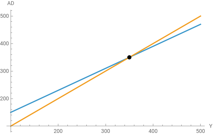
If the economy is in balance, this AD = 70 + 0.8Y must be met by the corresponding aggregate output-income, Y. That is to say, AD = Y .The solution is given by Y* = 350.
In[]:=
Solve[AD==Y,Y]
Out[]=
{{Y350.}}
The y-intercept of the AD curve is 70 and its slope is 0.8, whereas the Y curve starts from the origin with the slope of 1. The two lines intersect at the point of (Y*, AD*) = (350, 350) as in the graph below.
In[]:=
Plot[{70+0.8Y,Y},{Y,100,500},PlotLegends"Expressions",AxesLabel{"Y","AD"},Epilog{PointSize[Large],Point[{350,350}]}]
Out[]=


The government’s spending without taxes
The government’s spending without taxes
Let us now extend the previous model by introducing the government’s spending, G. Domestic aggregate demand is augmented by this additional spending component. That is, AD = HHC + PBI + G. For now we continue to ignore the possible changes in households consumption behavior induced by the tax payment obligation.
Following the same procedure, we can determine the equilibrium value of Y given AD = a+b*Y + PBI + G:
In[]:=
Clear[Y,AD,a,b,PBI,G];Solve[a+bY+PBI+G==Y,Y]
Out[]=
Y
-a-G-PBI
-1+b
Suppose now that we have the following numerical value for each component in this model. The modified AD and the corresponding equilibrium Y become:
In[]:=
Clear[AD,HHC,PBI,Y,C0,C1];AD=HHC+PBI+G;HHC=a+bY;a=50;b=0.8;PBI=20;G=50;
In[]:=
ADSolve[AD==Y,Y]
Out[]=
120+0.8Y
Out[]=
{{Y600.}}
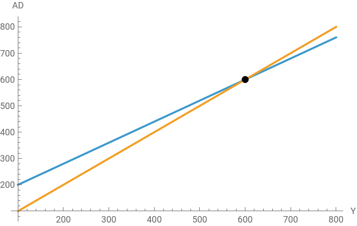
The y-intercept of the AD curve is now 120 and its slope is 0.8, whereas the Y curve starts from the origin with the slope of 1.
The two lines intersect at the point of (Y*, AD*) = (600, 600) as in the graph below.
The two lines intersect at the point of (Y*, AD*) = (600, 600) as in the graph below.
In[]:=
Plot[{120+0.8Y,Y},{Y,100,800},PlotLegends"Expressions",AxesLabel{"Y","AD"},Epilog{PointSize[Large],Point[{600,600}]}]
Out[]=
The government spending with the lump sum tax regime
The government spending with the lump sum tax regime
The previous model can be easily modified by considering the government’s tax revenue (T) and income transfer (TR). If the government imposes a lump sum tax on income (a certain fixed target tax revenue), while providing transfer income to needy households, we need to modify the households’ consumption spending flow accordingly. The following equations show this change:
AD=HHC+PBI+GHHC=a+b(Y-T+TR)AD=Y
Notice that the households consumption spending becomes a function of disposable income, Yd = Y-T+TR, which is adjusted by the tax payment obligation and the government’s subsidized income.
Following the same procedure, we can determine the equilibrium value of Y given AD = a + b(Y-T+TR) + PBI + G:
In[]:=
Clear[Y,AD,a,b,T,TR,PBI,G];Solve[a+b(Y-T+TR)+PBI+G==Y,Y]
Out[]=
Y
-a-G-PBI+bT-bTR
-1+b
Suppose now that we have the following numerical value for each component in this model. The modified AD and the corresponding equilibrium Y become:
In[]:=
Clear[AD,HHC,PBI,Y,C0,C1];AD=HHC+PBI+G;HHC=a+b(Y-T+TR);a=50;b=0.8;T=100;TR=10;PBI=20;G=50;
In[]:=
ADSolve[AD==Y,Y]
Out[]=
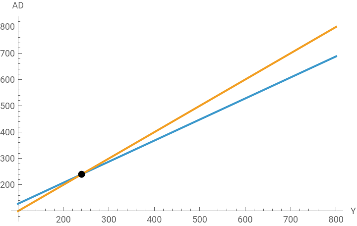
120+0.8(-90+Y)
Out[]=
{{Y240.}}
In[]:=
Plot[{120+0.8(Y-90),Y},{Y,100,800},PlotLegends"Expressions",AxesLabel{"Y","AD"},Epilog{PointSize[Large],Point[{240,240}]}]
Out[]=
The government spending with the marginal tax rate regime
The government spending with the marginal tax rate regime
Let us now consider the situation, in which the government imposes a certain fixed tax rate on income, as opposed to the fixed tax revenue in the previous case. In this situation, we have:
Notice that the households consumption spending is modified, and it becomes a function of disposable income, Y-tY+TR where t represents the average income tax rate on income. Compared to the previous case, the government is now collecting tax revenue flexibly, tying the total tax revenue to the change in aggregate output-income. Given tax rate, t, we can easily anticipate that total tax revenue for the government sector will rise if the economy is booming; conversely, the government’s total tax revenue will fall if the economy enters a recession and GDP falls.
Following the same procedure, however, we can continue to determine the equilibrium value of Y given AD = a + b(Y-tY+TR) + PBI + G:
Suppose now that we have the following numerical value for each component in this model. The modified AD and the corresponding equilibrium Y become:
From an algebraic point of view, the presence of the marginal tax rate lowers the multiplier, thereby preventing excessive swings and adjustments in aggregate output-income. For this reason, the government’s careful design for the marginal tax rate can stabilize the macroeconomic activity. Economists call this tax system an ‘automatic stabilizer.’
The international trade extension
The international trade extension
Using the same marginal tax rate regime case, let us now introduce both export and import component in aggregate demand. Let X denote the total volume of export, while M the volume of import. Then the model can be represented by the following set of equations:
Notice that the households consumption spending is made on both domestically produced goods and services and imported goods and services. The total volume of import is in this way estimated by the product of b2, the marginal propensity to consume for imported goods and disposable income. Since b2 represents households’ spending habits made on imported goods and services, the parameter b1 now represents households’ marginal propensity to consume for domestically produced goods and services.
With these modifications, we can find the equilibrium value of Y given AD = a + b1(Y-tY+TR) + PBI + G + X - b2(Y-tY+TR):
Suppose now that we have the following numerical value for each component in this model. The modified AD and the corresponding equilibrium Y become:
A difference equation model
A difference equation model
Introduction
Introduction
Up until now, we have reconstructed Keynes’s AD model using simple linear algebra. From now on, we build a dynamic model using both difference and differential equations.
The difference equation model and its analytical solution
The difference equation model and its analytical solution
If b < 1 or log(b) < 0, the solution monotonically converges to its steady state value. Otherwise, it diverge away from its steady state value.
A numerical example and visualization
A numerical example and visualization
Suppose we have a = 50, b = 0.8, PBI = 20, and G = 50. If the initial value of Y, Y(0) = 100, the numerical solution for this equation is:
The limit toward which this solution curve converges can be found by computing:
The following graph shows the behavior of the solution curve of Y[t]: It grows exponentially starting from its initial value of Y[0]=100:
A differential equation model
A differential equation model
The differential equation model and its analytical solution
The differential equation model and its analytical solution
We can replicate the same behavior of both AD and Y in a differential equation model. Suppose that the change in aggregate output-income over time is induced by the force that closes the gap between aggregate demand and aggregate output-income. We can write the following differential equation model:
where α is an adjustment parameter.
This is a linear first-order differential equation with a constant coefficient of α, a, and b. The solution to this equation can be found by using DSolve[] as follow:
As before, we can conduct a basic stability analysis of the solution curve. If the value of b is smaller than 1, the solution curve converges to the steady state value with α > 0. The higher value of α, the faster the adjustment toward its steady state value of the equation.
A numerical example and visualization
A numerical example and visualization
Now suppose a = 50, b = 0.8, PBI = 20, and G = 50. If the initial value of Y, Y(0) = 100 and α = 1.5, the numerical solution for this equation is:
The qualitative behavior of the solution curve remain the same as in the difference equation model.
Before closing, we can also visualize the changing behavior of the solution curve by changing the value of the adjustment parameter α in the following way:
Conclusion
Conclusion
The original AD model focuses on the importance of the change in aggregate demand and how this change affects the macroeconomic outcome measured by aggregate output-income. The spending-output multiplier, in which the marginal propensity to consume plays a crucial role, governs the behavior of the change in AD and Y. This note shows how we can construct this model in both linear and dynamic model setting.
There are some obvious limitations in AD models. For example, there is no consideration of the growth of the capital stock that must be affected by the constant private business investment spending. If there is a constant private business investment spending as in this model, there must be a corresponding change in the productive capital stock given a certain depreciation. But the AD model presented in this note does not account for this capital stock accumulation.
The same is true for the government’s budget. The government’s spending influences the current level of aggregate demand. But this public spending must be recorded in the government’s balance sheet that is jointly determined by its tax revenue. If the government spends more than its tax revenue, this deficit spending will accumulate the public debt over time. Unfortunately, none of these variables is fully explained in this baseline model.
Finally, it will be more insightful if we extend the baseline model by introducing a certain investment behavior: The private business investment spending can be a function of the past aggregate output-income as well as the cost of borrowing fund for investment spending. We can easily introduce the investment sensitivity to the change in either past consumption or aggregate output-income along with the change in the cost of borrowing. Some monetary variables such as money supply, the average long-term interest rate on corporate borrowing will also affect this investment sensitivity.
References
References
◼
John M. Keynes, The General Theory of Employment, Money and Interest. New York: Prometheus Books, 1997 [1936].
◼
Neva Goodwin et. al., Macroeconomics in Context, New York and London: Routledge, 2023 (The 4th edition)
◼
Ronald Shone, An Introduction to Economic Dynamics, Cambridge University Press: 2001, pp.48-60.
◼
Srinivas Raghavendra and Petri T. Piiroinen, An Introduction to Economic Dynamics - Modelling, Analysis and Simulation, Routledge: 2023, pp.47-60.
CITE THIS NOTEBOOK
CITE THIS NOTEBOOK
Introduction to dynamic economic models: Keynes's aggregate demand (AD) models
by Hee-Young Shin
Wolfram Community, STAFF PICKS, December 9, 2025
https://community.wolfram.com/groups/-/m/t/3588042
by Hee-Young Shin
Wolfram Community, STAFF PICKS, December 9, 2025
https://community.wolfram.com/groups/-/m/t/3588042