Self driving electric delivery trucks are key components of future urban infrastructure. Through this project, the optimization of delivery routes for these different trucks were explored in different scenarios- attempting to cover as many edges as possible while covering the least distance. Using Open Street Map Data, the graph analysed was that of a small neighbourhood in New York City by using junctions and roads to create edges and vertices. The algorithm explores partitioning the graph into components and finding the most optimal tour within those partitions for cases of 1,2,3, and k trucks. It was found that in general, as the number of trucks increased the delivery route became more optimised- covering less distance per truck and total distance overall.
Introduction
Introduction
Self-driving delivery trucks are emerging as a key component of future urban infrastructure, with their numbers projected to increase tenfold between 2022 and 2030. The idea behind these trucks is that they start and end at the same point, forming a closed route. This project explores the routes that self-driving trucks could take—whether using 1 truck, 2 trucks, or k trucks—and explores the configurations that reduces the total distance covered while ensuring every street in a specific New York neighborhood is visited. Using concepts such as Chinese Postman Tours, which ensure every edge in a graph is covered thus covering all the houses/ buildings in all the streets, the project investigates the routes delivery trucks would need to follow. It also considers limitations in the partitioning method, identifying missing edges that, if added, create more optimal subgraphs. Overall, this project examines the most efficient routing strategies for autonomous delivery trucks.
The project explores the following areas:
1. Importing and processing data
2. Establishing junctions and roads in the graph as vertices and edges
3. Finding the optimum path for only one truck
4. Optimum path for two trucks – no missing roads considered
5. Optimum path for two trucks – missing roads considered without verifying correct combinations
6. Optimum path for two trucks – missing roads considered with correct combinations
7. Optimum path for three trucks – no missing roads considered; edge weights included; distance calculated for all three trucks
8. Generalized k-truck routing – Extending the approach to any number of trucks, with distances calculated per truck and total system distance evaluated.
Importing data and processing
Importing data and processing
The data used for this algorithm was sourced from open-source map data, which includes geographic locations and classifications of entities such as roads, pavements, and buildings. This dataset was chosen for two key reasons: first, roads could be easily extracted for focused analysis; second, the inclusion of geographic coordinates enabled straightforward calculation of edge weights based on real-world distances in later stages of the algorithm.
In[]:=
osm=ResourceFunction["OSMImport"]
Out[]=
OSM data can only take in a limited geographic area therefore only a small block/ neighbourhood is being explored in this algorithm.
Establishes the boundaries for the New York City neighbourhood
In[]:=
bounds={{40.6982,40.72190},{-73.96108,-73.9569}};
Imports the position for the coordinates and ways in the neighbourhood from open street map data.
In[]:=
osmNYCImport=osm[GeoBoundsRegion[bounds]]
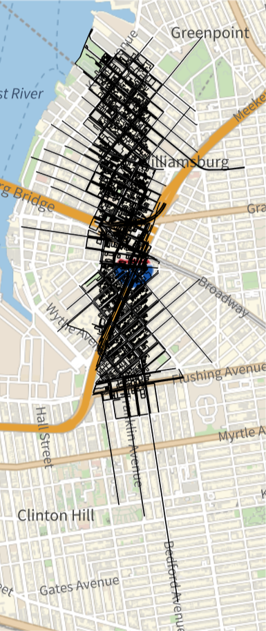
Checks the geographic region to see if it is near a water body and the junctions
In[]:=
GeoGraphics[Values[Line[Values[osmNYCImport[["Nodes",#Nodes,"Position"]]]]&/@osmNYCImport["Ways"]]]
Out[]=
In[]:=
nodePositions=osmNYCImport[["Nodes",All,"Position"]]
Selects all roads in the dataset
In[]:=
tempRoads=osmNYCImport["Ways"]
Extracting vertices and edges for the graph
Extracting vertices and edges for the graph
The keynodes specifies the nodes and their associated ID Keynodes List extracts only the nodes for the keynodes list .
In[]:=
keynodes=tempRoads[[All,"Nodes"]];keyNodesList=Values[keynodes];
Function for finding the position of the endpoints of each junction from the bigger list of nodes :
In[]:=
end=Flatten[Table[{{i,1},{i,Length[keyNodesList[[i]]]}},{i,Length[keyNodesList]}],1]
Function finds the endpoints of the ways to find the junctions and create the edge list for the graph which will be reconstructed:
In[]:=
findEndNodePosition[endpoint_]:=Position[Values[keynodes],#]&/@{endpoint[[1]],endpoint[[-1]]}endpointpositions=findEndNodePosition/@keyNodesList
Segregates the end points so that it is ordered by the junctions closest to each other by index number and deletes any junctions which may be duplicated in the process .
In[]:=
end=DeleteDuplicates[SortBy[Flatten[endpointpositions,2],1]]
Finds all the duplicates which exist in more than 1 road- at intersections and then deletes duplicates of those intersection positions:
In[]:=
getJunction[x_]:=DeleteDuplicates[ResourceFunction["Duplicates"][Flatten[x]]];nodesList=getJunction[Flatten[keyNodesList]];
nodesPositions gives the index positions of the junction values which were found
In[]:=
nodesPositions=DeleteDuplicates[Join[Flatten[Position[keyNodesList,#]&/@nodesList,1],end]]
Index positions organises the node positions so that the ones which have the same starting index are grouped together .
In[]:=
indexPositions=GatherBy[nodesPositions,#[[1]]&]
Joins the ends of the ways which are junctions with junctions which intersect more than one way - giving all the vertices of the graph
Sorted indexes sorts all the junction positions so they are all one after the other .
Sorted indexes sorts all the junction positions so they are all one after the other .
In[]:=
sortedIndexes=SortBy[Map[SortBy[#,Last]&,indexPositions],First]
sortedAll creates smaller sublists of 2 for the junctions to be interconnected
In[]:=
sortedAll=Partition[#,2,1]&/@sortedIndexes
Splitting the nodes at the indexed positions (junctions) for the 1 st set of way data . The function is used for sorting through the algorithm for the rest of the data . getWaysSegments creates a new function to split the nodes at the index positions specified .
In[]:=
getWaySegments[way_,pairs_]:=way[[#[[1,2]];;#[[2,2]]]]&/@pairs
Nodes applies the function getWaySegment so that the nodes are all split at the sorted paths
In[]:=
nodes=Table[getWaySegments[keyNodesList[[i]],sortedAll[[i]]],{i,1,Length[keyNodesList]}]
The variable newEdges creates smaller sublists of the first and last elements in the sublists of edges therefore creating edges so that smaller vertexes which are not edges are not included, reducing the number of unnecessary edges included in the code .
In[]:=
newEdges=Map[{#[[1]],#[[-1]]}&,Flatten[nodes,1]]
Creating graphs and subgraphs for exploration
Creating graphs and subgraphs for exploration
Creates a graph of the neighbourhood being worked with which is further split as the graph is too large to process entirely.
In[]:=
fullNeighbourhoodGraph=Graph[UndirectedEdge@@@DeleteDuplicates[newEdges],VertexSize->0.1];
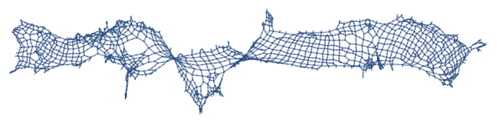
Because of the limitations of OSM data which does not cover every intersection and roads, now, we need to find the graph components which are completely connected to each other through edges- ignoring streets that have no connections between them on open street map data. newNeighbourhood considers a smaller area within the neighbourhood which is connected together. The variable positionsOfNodes finds the position of the vertexList of the newNeighbourhood graph within the keyNodesList list. firstLast finds the first and last positions of the sublists within the vertex list to find the endpoints of the junctions.
In[]:=
subGraphs=ConnectedGraphComponents[fullNeighbourhoodGraph];newNeighbourhood=subGraphs[[1]]vertexes=VertexList[newNeighbourhood];edge=EdgeList[newNeighbourhood];positionsOfNodes=Map[Position[keyNodesList,#]&,vertexes];firstLast=Map[{#[[1]],#[[-1]]}&,positionsOfNodes];
Out[]=
Geopos finds the node positions of the edges . And geos yields the coordinates of the geopos node positions. This is needed for creating edge weights using distance between the two junctions so that path can follow the shortest distance everytime.
In[]:=
geoPositionOfNodes=nodePositions[[#]]&/@Flatten[firstLast,1];geos=Values[geoPositionOfNodes];
Finds the distance between the junction and dis converts all the units to a standard miles so the edge weight is more accurate.
In[]:=
distance=GeoDistance[#]&/@geos;distanceBetweenWeights=QuantityMagnitude[Map[UnitConvert[#,Quantity["Miles"]]&,distance]];
In[]:=
new=Graph[EdgeList[newNeighbourhood],GraphLayout->"GridEmbedding",EdgeWeight->distanceBetweenWeights[[;;Length[EdgeList[newNeighbourhood]]]],EdgeLabels->"EdgeWeight"];new1=Graph[EdgeList[newNeighbourhood],GraphLayout->"GridEmbedding"]
Out[]=
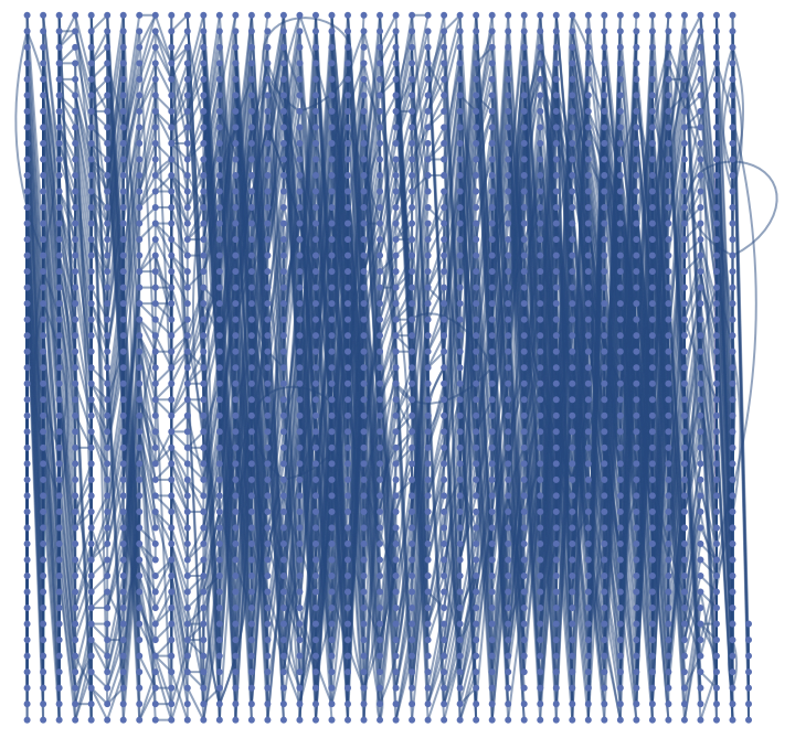
Creates a list of associations applying the edge weight to every distanceBetweenWeightstance calculated thus every 2 edges have a edge wieght based off its distanceBetweenWeightstance.
In[]:=
edgeDistanceAssociation=AssociationThread[EdgeList[new]->distanceBetweenWeights[[;;Length[EdgeList[new]]]]];
Optimizing the route for graph with 1 truck, no edge weights and no distanceBetweenWeightstances included.
Optimizing the route for graph with 1 truck, no edge weights and no distanceBetweenWeightstances included.
This section visualises the simplest postman tour for covering from 1 to all edges for a singular truck without any clustering.
In[]:=
step1=FindPostmanTour[newNeighbourhood][[1]];
Creates a user interface where the user can chose the path size they want and check the shortest route from that path back to the starting point which is index 1 of the random graph .
Optimization of two trucks without edge weights and missing edges accounted for
Optimization of two trucks without edge weights and missing edges accounted for
This section explores visualisation of the postman tours for division of the graph into two clusters--one for each truck--and finding the optimal route for each cluster. We focus on optimizing each components’ individual tour to find a globally maximal solution.
Choses two areas of newneighbourhood, the small section of new york city data which are approximately equal in size.
interEdges extracts the edges which are not in either subgraph- the missing edges in between the two graphs which were removed during the process of graph partitioning.
Creates the edge list of subGraphs 1 and 2 to add the missing edges to .
Combines missing edges in various different arrangements for appending to the edge lists .
results creates twoPartitions table where the edge list of the first subgraph and the missing edges are connected along with the second subgraph and the missing edges are connected . Furthermore, g1 and g2 creates graphs for appending the vertex list of the subGraphs to the new edge list with the missing edges thus ensuring that every edge is connected to twoPartitions vertex on the subGraphs and ensuring edges are covered in subGraphs .
Summary function to find PostmanTours for all permutations of graphs and then return the total distance covered by each:
Visualization of the optimally short path, covering most edges:
However the limitation of this algorithm is that it does not take into account the correct combinations of missing edges . It finds the missing edges combination for each subgraph individually without taking into consideration that the two subGraphs could cover all edges thus repeating some edges and some subGraphs may not cover all possible missing edges . It shows the optimized graph for 2 clusters with random combinations . Meaning that if there are 5 missing edges, the shortest tour may be for 3 missing edges and another subgraph shortest tour may be 3 missing edges as well . The correct combinations of the edges which are missing from the subgraphs are not accounted for .
Optimization of 2 trucks by clustering and iterating though every missing vertexes.
Optimization of 2 trucks by clustering and iterating though every missing vertexes.
This section develops an algorithm for matching the correct combinations of the missing edges between the two clusters without taking edge weight into account yet .
Extracts the edge list of the subgraph which is explored
Creating the subGraphs for shortest paths which do not account for the combinations of missing vertexes and subGraphs
Creating the subGraphs for shortest paths which do not account for the combinations of missing vertexes and subGraphs
Partitioning creates two sections so that the two components are as equal in area as possible for graphs without edge weights. Because of this, we use it to create two semi-equal components so that the cycles are not incredibly spanning and inefficient.
Partitioning used to cluster the graphs
Finds the edges in the bigger graph which are not in any graph clusters which have been created
subsetCombos1 creates all the possible combinations of the missing edges and how they can be arranged.
Now, we have the summary function to execute the algorithm. The results Table creates twoPartitions table where the edge list of the first subgraph and the missing edges are connected along with the second subgraph and the remaining missing edges which the 1st graph did not cover are connected as shown through the Append function. Furthermore, g1 and g2 creates graphs for appending the vertex list of the subGraphs to the new edge list with the missing edges thus ensuring that every edge is connected to twoPartitions vertex on the subGraphs and ensuring edges are covered in subGraphs. PostManTour finds the various postman tours within the various g1 and g2 graphs. Furthermore, the MinimalBy function finds the smallest postman tour within the various postman tours the smallest one thus giving the graph which covers the least distanceBetweenWeightstance in total.
Uses the euclidean distance to find the closest edges however does not take physical distance between the edges into account.
Shows the optimal path between the two clusters which also shows twoPartitions few missing vertexes as highlighted in light blue .
Creating the subGraphs for shortest paths which account for the combinations of missing vertexes and subGraphs
Creating the subGraphs for shortest paths which account for the combinations of missing vertexes and subGraphs
To address the limitations of the previous method, the next approach pairs the edges as follows: if one subgraph has 2 missing edges connected, the other subgraph takes the remaining 3 connected edges. This ensures the path is more realistic and that every missing edge is included, while avoiding any edge being used twice by the same subgraph. All possible edge combinations within the edge list are considered. For example, if the missing edge list is {a, b, c}, this method explores assigning {a} to subgraph 1 and both {b, c} and {c, b} to subgraph 2 to find the most efficient path.
se1 and se2 creates edgelists for the individual subgraphs
moremissing finds the missing edges which are in neither edge list
Highlights the parts of the neighbourhood which are not included in the subgraph clusters.
Finds the various different combinations of the missing edges.
Joins the edge list of the different combinations of missing edges with the edge list of the two clusters.
Now the algorithm which covers all the missing edges and takes into account the right combination is explored through a summary table module function. The allAssignments variable generates all possible subsets of the moremissing edge list. The tourResults table creates twoPartitions table where the edge list of the first subgraph and the missing edges are connected, along with the second subgraph and the remaining missing edges which the first graph did not cover, as shown through the Join function. Specifically, for each subset twoPartitions, e1 is formed by joining enlist1 with twoPartitions, and e2 is formed by joining enlist2 with Complement[moremissing, twoPartitions]. The Complement function ensures that the remaining edges not included in twoPartitions are assigned to the second subgraph, so that every edge in moremissing is covered exactly once and the correct combinations are followed. Furthermore, g1 and g2 create graphs by appending the vertex list of the subgraphs to the new edge lists with the missing edges, thus ensuring that every edge is connected to twoPartitions vertex on the subgraphs and all missing edges are included. FindPostmanTour finds the postman tours within the various g1 and g2 graphs. The result for each subset twoPartitions includes the subset, both tours, and the combined length of both tours. Finally, the MinimalBy function finds the smallest postman tour within the various combinations, thus giving the graph configuration which covers the least total distance.
Finds the shortest postman tour for all possible combinations of subGraphs with the vertexes connected together.
United graph shows the visualisations of the three subgraphs recombined into twoPartitions singular huge graph. It is used later for finding the missing edges which were unaccounted for while the partitioning happened.
Three Clusters Method
Three Clusters Method
This algorithm takes the physical distance between junctions into consideration to reduce the total distance being travelled by each of the three trucks by setting the distance extracted from the nodes with OSM data as the edge weights. It finds the shortest Postman Tour by calculating distance and finding the route with the smallest distance covered .
This algorithm starts by clustering the neighbourhood into parts through edge weights (distanceBetweenWeightstances) by Graph Partition so the least distance is covered.
Finds graph partitions and saves each of them to a subgraph:
Shows the division of the three clusters on the bigger graph and shows that there are missing edges which is an issue solved in the later stages.
Postmantours function creates a map to find the smallest distanceBetweenWeightstance being covered within the individual tour for twoPartitions cluster of 3.
Sortedlistofedges sorts the edgelist of the postmanparts so the ones that are closer to each other are arranged together.
Checks whether the three subgraphs are connected as that is a requirement for obtaining the postman tours of the seperate graphs which are obtained later.
SortedVertex2 finds the vertex list of each postman tour and formats it so that it matches the formatting of the association edgeDistanceAssociation to find matching components-this will be used to find the edge weights of individual postman tours.
Finding the missing vertexes
keyList is used to split the bigger edgeDistanceAssociation association so it is divided into smaller parts which match the format of the undirected edges
Finds the position of the directed edges in reverse and normalVertexVertex in the bigger association of keys.
Deletes the empty cells within the list
Extracting the distance travelled by each path in the third cluster as well as the total distance travelled by dividing the path into three junctions .
tourPositions is used find the positions of weight of every edge in the tours and tourweights uses these positions to find the total of the edge weights for each postman tour. Total of the tourweights gives the total distance travelled by all 3 postman tours in the whole three clusters method.
Generalised clustering method for k number of clusters
Generalised clustering method for k number of clusters
Asks the user to input how many partitions, aka trucks which cover the neighbourhood
Accordingly partitions the graph into k number of sections accounting for the minimal edge weight in these distances .
Finds postmantours for the individual partitions within the k partitions and produces the edge list for the same:
kpos1 ensures that the smaller node is before the larger node so the undirected edges are arranged in the same way and can be directly compared to the keys in the first association edgeDistanceAssociation without having to reverse the edges to compare.
Extracting the distance travelled by each path in the third cluster as well as the total distanceBetweenWeightstance travelled by dividing the path into three junctions .
ktourPositions is used find the positions of weight of every edge in the tours and tourweights uses these positions to find the total of the edge weights for each postman tour . Total of the ktourweights gives the total distance travelled by all 3 postman tours in the whole three clusters method .
Conclusion
Conclusion
For 4 clusters, the total distance covered significantly decreases from 203.471 in 3 clusters to 111.15 for 4 clusters . The postman tour length significantly decreases and when accounting the individual edge weights/ distances into the formula, the individual clusters have a range of distances that they cover which are not equal. This shows that graph partitioning through this method works by taking individual cluster distances into account and reducing the overall distance covered in the clusters altogether. The clustering method increases the optimization of the self driving electric service trucks by decreasing overall distance covered while covering all the edges.
Citations
Citations
1
.Welcome To Zscaler Directory Authentication. (2025). Patentpc.com. https://patentpc.com/blog/self-driving-delivery-vehicles-market-expansion-adoption-rates-and-growth-trends
2
.Hölscher, A. (n.d.). A Cycle-Trade Heuristic for the Weighted k-Chinese Postman Problem. Retrieved July 10, 2025, from https://liu.diva-portal.org/smash/get/diva2:1275190/FULLTEXT01.pdf
Future Directions
Future Directions
I would love to keep working on this project so it can be used in a more generalized manner for any randomized neighbourhood in the world for a more broad application of the uses. Furthermore, more constraints could be integrated into the algorithm for the trucks to find out the optimum number of trucks which could adhere to these constraints while finding an optimal path. Looking into cost analysis of these distances as well for the various trucks would have also been more interesting to explore.
I would love to keep working on this project so it can be used in a more generalized manner for any randomized neighbourhood in the world for a more broad application of the uses. Furthermore, more constraints could be integrated into the algorithm for the trucks to find out the optimum number of trucks which could adhere to these constraints while finding an optimal path. Looking into cost analysis of these distances as well for the various trucks would have also been more interesting to explore.
Acknowledgements
Acknowledgements
I would like to thank my mentor Zoya Brahimzadeh for guiding me continuously throughout the process . As well as the teaching assistants including Damla for giving me support when needed . Thank you to the WSRP staff for giving me the opportunity to develop this project .
CITE THIS NOTEBOOK
CITE THIS NOTEBOOK
Optimizing travel routes for self driving electric trucks in a New York neighbourhood
by Anwesha Mazumdar
Wolfram Community, STAFF PICKS, July 10, 2025
https://community.wolfram.com/groups/-/m/t/3502974
by Anwesha Mazumdar
Wolfram Community, STAFF PICKS, July 10, 2025
https://community.wolfram.com/groups/-/m/t/3502974