Applications of the Soave-Redlich-Kwong Equation of State
Authors: Housam Binous and Ahmed Bellagi
Applications of the Soave-Redlich-Kwong Equation of State
Authors: Housam Binous and Ahmed Bellagi
Authors: Housam Binous and Ahmed Bellagi
One can use the Soave - Redlich - Kwong Equation of State to compute vapor and liquid molar volumes and vapor pressure at various temperatures as well as the vapor liquid equilibrium curve for Ethane . The vapor pressure data obtained using this cubic equation of state is compared with success to the results derived from the modified Antoine' s equation .
Acknowledgement :
This problem was presented in the Master's report of R. Privat under the direction of J-P Corriou.
This problem was presented in the Master's report of R. Privat under the direction of J-P Corriou.
In[]:=
θ=.;
In[]:=
Off[NIntegrate::"nlim"]
In[]:=
Off[General::"spell1"]
Reduced Temperature
In[]:=
Tre=(θ+273.15)/Tc;
Ethane's Critical Pressure, Critical Temperature and Accentric Factor. R is the Universal Gas Constant
In[]:=
Tc=273.15+32.28;Pc=48.84;ω=0.09860;R=83.14;
Soave-Redlich-Kwong Equation of State
In[]:=
P[T_,v_]:=RT/(v-b)-a/(v(v+b))
In[]:=
b=0.08664RTc/Pc
Out[]=
45.0469
In[]:=
m=0.480+1.574ω-0.176ω^2
Out[]=
0.633485
In[]:=
a=0.42748(RTc)^2/Pc1+m1-
Tre
^2Out[]=
5.64396×
6
10
2
1+0.6334851-0.0572195
273.15+θ
In[]:=
tbl=Table[P[θ+273.15,v],{θ,1,30,5}];
Plotting Isotherms
In[]:=
plt[θ_]:=Plot[tbl[[θ]],{v,0,2500},PlotRange{{0,2500},{0,100}},PlotStyleHue[θ/6],DisplayFunctionIdentity]
In[]:=
plot1=Show[Table[plt[θ],{θ,1,6}],DisplayFunction$DisplayFunction]
Out[]=
Finding vapor pressure and liquid and gas molar volumes at different temperatures. Dots in the figure show vapor liquid equilibrium curve for ethane.
In[]:=
sol[θ_]:=FindRoot[{NIntegrate[-P[273.15+θ,v]+P[273.15+θ,x],{v,x,z}]NIntegrate[P[273.15+θ,v]-P[273.15+θ,y],{v,z,y}],P[273.15+θ,x]P[273.15+θ,z],P[273.15+θ,z]P[273.15+θ,y]},{x,50},{z,120},{y,400},MaxIterations->100]
In[]:=
tbl1=Table[{x/.sol[θ],P[θ+273.15,x/.sol[θ]]},{θ,1,30,5}]
Out[]=
{{85.1397,24.8124},{89.1129,27.9134},{93.9325,31.2787},{99.9972,34.9205},{108.085,38.8506},{120.123,43.0813}}
In[]:=
tbl2=Table[{y/.sol[θ],P[θ+273.15,y/.sol[θ]]},{θ,1,30,5}]
Out[]=
{{629.251,24.8124},{543.734,27.9134},{468.08,31.2787},{400.224,34.9205},{338.019,38.8506},{278.409,43.0813}}
In[]:=
TBL=Join[tbl1,Sort[tbl2]]
Out[]=
{{85.1397,24.8124},{89.1129,27.9134},{93.9325,31.2787},{99.9972,34.9205},{108.085,38.8506},{120.123,43.0813},{278.409,43.0813},{338.019,38.8506},{400.224,34.9205},{468.08,31.2787},{543.734,27.9134},{629.251,24.8124}}
In[]:=
plot2=ListPlot[TBL,PlotStylePointSize[0.025]]
Out[]=
In[]:=
Show[plot1,plot2,PlotRange{{0,600},{5,50}}]
Out[]=
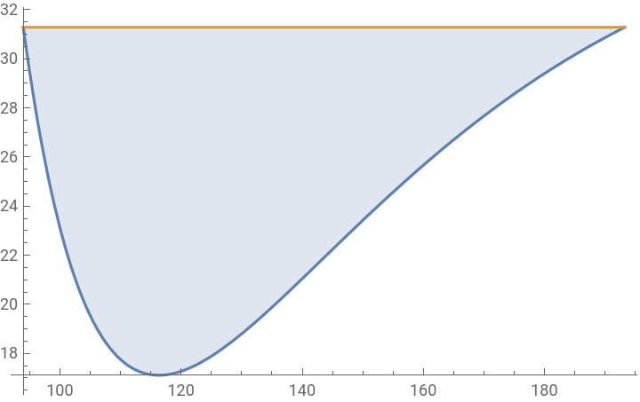
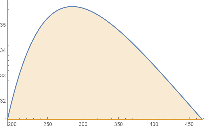
The equilibrium data is obtained by solving a system of equation so that the two areas are equal.
In[]:=
θ=11;
In[]:=
sol11=sol[11]
Out[]=
{x93.9325,z193.269,y468.08}
In[]:=
plt5=Show[plt[3],Epilog{Line[{{x/.sol[11],P[11+273.15,x/.sol11]},{y/.sol[11],P[11+273.15,y/.sol11]}}],{PointSize[0.025],Point[{y/.sol[11],P[11+273.15,x/.sol11]}],Point[{x/.sol11,P[11+273.15,x/.sol11]}],Point[{z/.sol11,P[11+273.15,x/.sol11]}]}},PlotRange{{0,600},{5,50}}]
Out[]=
In[]:=
NIntegrate[(-P[273.15+θ,v]+P[273.15+θ,x])/.θ11,{v,x,z}]/.sol[11]
Out[]=
772.277
In[]:=
NIntegrate[(P[273.15+θ,v]-P[273.15+θ,y])/.θ11,{v,z,y}]/.sol[11]
Out[]=
772.277
In[]:=
plt7=Plot[{P[θ+273.15,v]/.θ11,P[273.15+θ,y]/.θ11/.sol11},{v,x,z}/.sol11,Filling{1{2}}]
Out[]=
In[]:=
plt8=Plot[{P[θ+273.15,v]/.θ11,P[273.15+θ,y]/.θ11/.sol11},{v,z,y}/.sol[11],Filling{2{1}}]
Out[]=
Vapor pressure data versus temperature. Comparison with experimentally derived expressions of vapor pressure. We get a perfect fit with the modified Antoine's equation.
Modified Antoine's equation obtained from HYSYS 3.2
Antoine's equation obtained from Equilibrium-Stage Separation Operations in Chemical Engineering by Henley and Seader, Wiley, 1981.