Setup
Setup
Introduction
Introduction
A Turing machine is a simple model of computation that is able to run any program any real computer can run, in principle. For instance, here is a paper by researcher Greg Michaelson, “A Turing Machine For SKI Combinators,” that describes how to implement SK combinator calculus with a Turing Machine, which can then implement lambda calculus, (here is a link to some Wolfram Language code to do this step, from A New Kind of Science again) from which one can start building up a practical programming language (for instance, the actual practical functional programming language Haskell is built up from lambda calculus.)
There are many systems that are very simple that one might want to prove Turing complete, such as rule 110. But to show such systems Turing complete, one has to essentially build some other Turing complete system within them. Turing machines, while simple, are still somewhat complex to emulate in some systems which don’t have things Turing machines have like multiple symbols, a or a separate head that can move back and forth and store and compare symbols, or an infinite tape. So one wants to find an even simpler system. It turns out that a certain other Turing complete system called cyclic tag is so simple that many other systems have been shown Turing complete by emulating that, the cyclic tag system.
But the bridge must be built from which one can run a Turing machine on a cyclic tag system to show that cyclic tag itself is Turing complete.
To do so, one can go through a series of emulations, such as one that happens to be shown in Stephen Wolfram’s book A New Kind of Science, in which one emulates in this order, Turing Machine with arbitrary number of symbols -> Turing machine with only two symbols -> Tag system -> Cyclic tag system. A description of this chain of emulations is described in 4 pages of text and images here. There’s just one issue with that version though, which is that it goes through a step, going from Turing machine which two symbols to tag system in which integers of arbitrary size are encoded in unary. This means that emulated programs can get exponentially large and slow.
Fortunately, there was later found a way to get around this. Unfortunately, that way is much more complicated, and is described in a 2009 paper, “A Concrete View of Rule 110 Computation” by Matthew Cook and also a 2006 paper by Turlough Neary and Damien Woods. The new route, which avoids using unary, goes Turing machine with arbitrary symbols -> something called a “clockwise Turing machine” (with arbitrary symbols) -> clockwise Turing machine with only two symbols on the tape (though arbitrary number of head symbols) -> Tag system -> cyclic tag system. The trickiest step is definitely the one from clockwise Turing machine -> tag system.
However, while the algorithm is described in those papers, I was unable to find an actual implementation of that algorithm. So I implemented it in code myself based off the slightly more concrete description in the 2009 paper. I’ve included an attachment with all the files, and algorithms. To run it, download the attached files, along with this notebook, put them all in the same folder, and then run this notebook. Below however is just showing how each step of emulation works, one at a time, by just showing the rules for emulating one system with the other, and comparing the two systems running with one emulating the other. All of the emulation steps below I wrote based off descriptions from the paper, except for the last step, tag -> cyclic tag, which is just slightly modified code from A New Kind of Science.
Turing Machine to Clockwise Turing Machine
Turing Machine to Clockwise Turing Machine
A Turing machine has an infinite tape with symbols on it, and a “head” that can be in some state and move left or right depending on what state the head is in, and what symbol it’s “looking at” at the time. The head compares its state to the symbol on the tape, writes a new symbol, then changes and moves left or right before doing this all over again. Simpler than most programming languages, and so simple enough to be a good model for computation and bridge from even simpler systems to more complex ones, but not as simple as some systems that come further that slowly do away with things like more than two symbols, heads, infinite tapes, and moving in more than one direction. So in this first step, we’re going to do away with the need for a Turing machine to have an infinite tape, by making it run instead on a clockwise Turing machine which uses a finite, but sometimes expanding tape.
Here is a specific Turing machine which happens to have the simplest rules that will still actually allow it to do any computation:
Here is a specific Turing machine which happens to have the simplest rules that will still actually allow it to do any computation:
In[]:=
tM=TuringMachine[{596440,2,3}];
In[]:=
RulePlot[tM]
Out[]=
Here it is running, starting with a blank tape. Time goes down the page, the orientation of the “tear drop” is the state of the head, and the colors represent symbols on the tape. (It starts as a tape with all one symbol, 0 or white here).
In[]:=
RulePlot[tM,{1,{{},0}},20,Mesh->All]
Out[]=
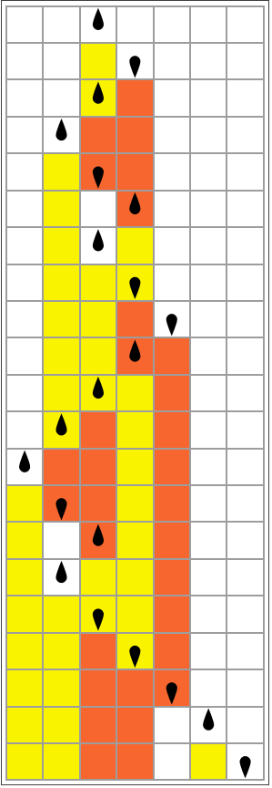
Here are the rules for that Turing machine in a more explicit form:
In[]:=
tMRule=ResourceFunction["ComputationalSystemRules"][tM]
Out[]=
{{1,2}{1,1,-1},{1,1}{1,2,-1},{1,0}{2,1,1},{2,2}{1,0,1},{2,1}{2,2,1},{2,0}{1,2,-1}}
Here, we have converted the rules for the Turing machine into the rules for a clockwise Turing machine that emulates the Turing machine. A clockwise Turing machine is a Turing machine where the tape is finite, cyclical, and the head only ever moves to the right (it can, however, add more than one symbol at a time to grow the tape).
In[]:=
tmToCWTMRule=TMToCWTM[tMRule]
Out[]=
Here you can see the CWTM running. The head state is the first integer in the list, and the tape is the list to its right. The tape itself just rotates to the right each time to show the head “moving”. The L and R states on the tape keep track of the left and right boundaries of the portion of the tape of the original non-clockwise Turing machine that has symbols (besides the “blank” background symbols) written on it.
It’s easiest to see that it is indeed emulating the above Turing machine by looking at states of the clockwise Turing machine that don’t have “Fl” in the head of the machine (those parts correspond to the Turing machine moving left and get a bit complicated) and to compare the tape of those non-FL parts to the parts of the original Turing machine where that machine is neither moving left, nor at a local leftmost position (is moving right or at a rightmost position). One should be able to see that the tape, when read in a loop from L to R, corresponds to the original, and that the heads correspond there also.
It’s easiest to see that it is indeed emulating the above Turing machine by looking at states of the clockwise Turing machine that don’t have “Fl” in the head of the machine (those parts correspond to the Turing machine moving left and get a bit complicated) and to compare the tape of those non-FL parts to the parts of the original Turing machine where that machine is neither moving left, nor at a local leftmost position (is moving right or at a rightmost position). One should be able to see that the tape, when read in a loop from L to R, corresponds to the original, and that the heads correspond there also.
In[]:=
cWTM[tmToCWTMRule,TMToCWTMInit[{1,{0}}],50]//Column
Out[]=
{1,{0,R,L}} |
{2,{R,L,1}} |
{Fl[1,R],{L,1,Ml,2}} |
{Fl[1,L],{1,Ml,2,R}} |
{Fl[1,1],{Ml,2,R,L}} |
{Fl[1,2],{2,R,L,Ml}} |
{Fl[1,2],{R,L,Ml,2}} |
{Fl[1,R],{L,Ml,2,2}} |
{Fl[1,L],{Ml,2,2,R}} |
{2,{2,2,R,L,1}} |
{1,{2,R,L,1,0}} |
{Fl[1,1],{R,L,1,0,Ml}} |
{Fl[1,R],{L,1,0,Ml,1}} |
{Fl[1,L],{1,0,Ml,1,R}} |
{Fl[1,1],{0,Ml,1,R,L}} |
{Fl[1,0],{Ml,1,R,L,1}} |
{2,{1,R,L,1,1}} |
{2,{R,L,1,1,2}} |
{Fl[1,R],{L,1,1,2,Ml,2}} |
{Fl[1,L],{1,1,2,Ml,2,R}} |
{Fl[1,1],{1,2,Ml,2,R,L}} |
{Fl[1,1],{2,Ml,2,R,L,1}} |
{Fl[1,2],{Ml,2,R,L,1,1}} |
{Fl[1,1],{2,R,L,1,1,Ml}} |
{Fl[1,2],{R,L,1,1,Ml,1}} |
{Fl[1,R],{L,1,1,Ml,1,2}} |
{Fl[1,L],{1,1,Ml,1,2,R}} |
{Fl[1,1],{1,Ml,1,2,R,L}} |
{Fl[1,1],{Ml,1,2,R,L,1}} |
{Fl[1,2],{1,2,R,L,1,Ml}} |
{Fl[1,1],{2,R,L,1,Ml,2}} |
{Fl[1,2],{R,L,1,Ml,2,1}} |
{Fl[1,R],{L,1,Ml,2,1,2}} |
{Fl[1,L],{1,Ml,2,1,2,R}} |
{Fl[1,1],{Ml,2,1,2,R,L}} |
{Fl[1,2],{2,1,2,R,L,Ml}} |
{Fl[1,2],{1,2,R,L,Ml,2}} |
{Fl[1,1],{2,R,L,Ml,2,2}} |
{Fl[1,2],{R,L,Ml,2,2,1}} |
{Fl[1,R],{L,Ml,2,2,1,2}} |
{Fl[1,L],{Ml,2,2,1,2,R}} |
{2,{2,2,1,2,R,L,1}} |
{1,{2,1,2,R,L,1,0}} |
{Fl[1,1],{1,2,R,L,1,0,Ml}} |
{Fl[1,1],{2,R,L,1,0,Ml,1}} |
{Fl[1,2],{R,L,1,0,Ml,1,1}} |
{Fl[1,R],{L,1,0,Ml,1,1,2}} |
{Fl[1,L],{1,0,Ml,1,1,2,R}} |
{Fl[1,1],{0,Ml,1,1,2,R,L}} |
{Fl[1,0],{Ml,1,1,2,R,L,1}} |
{2,{1,1,2,R,L,1,1}} |
Many State Clockwise Turing Machine to Two State Clockwise Turing Machine
Many State Clockwise Turing Machine to Two State Clockwise Turing Machine
The next step is to convert the many-state clockwise Turing Machine into a Turing machine with just two states on the tape (though it can still have any number of head states). I pick a particular simple multi state clockwise Turing machine and show how to convert that one into one that has only two states on the tape (however it can have an arbitrary number of head-states). Here is the rule for the machine:
In[]:=
cWTMRule={{1,0}{2,{0,1}},{2,0}{2,{2}},{3,0}{1,{0}},{1,1}{2,{0}},{2,1}{3,{1}},{3,1}{1,{0,0}},{1,2}{3,{0}},{2,2}{1,{2,2}},{3,2}{2,{1}}};
Here it is running:
In[]:=
cWTM[cWTMRule,{1,{0}},20]//Column
Out[]=
{1,{0}} |
{2,{0,1}} |
{2,{1,2}} |
{3,{2,1}} |
{2,{1,1}} |
{3,{1,1}} |
{1,{1,0,0}} |
{2,{0,0,0}} |
{2,{0,0,2}} |
{2,{0,2,2}} |
{2,{2,2,2}} |
{1,{2,2,2,2}} |
{3,{2,2,2,0}} |
{2,{2,2,0,1}} |
{1,{2,0,1,2,2}} |
{3,{0,1,2,2,0}} |
{1,{1,2,2,0,0}} |
{2,{2,2,0,0,0}} |
{1,{2,0,0,0,2,2}} |
{3,{0,0,0,2,2,0}} |
{1,{0,0,2,2,0,0}} |
Here are the rules where it has been converted into a 2 state machine:
In[]:=
coloredToBinCWTMRule=ColoredToBinCWTM[cWTMRule]
Out[]=
And here it is running. I show the head state on the left, and the tape state on the right.
Note that the head state is rather complex and does hold a good amount of information, but can still be considered one symbol (there could, for instance, just be one integer that represents each head state).
In the tape, symbols are converted into binary, but “padded” to all have the same length (whatever length the maximum symbol on the original CWTM tape needs). In this case, since the numbers in the original are 0-2, each symbol in the binary one needs two symbols. Since it needs two symbols, each step of the original CWTM needs a corresponding 2 steps in the binary CWTM (we’ll call this number X for now).
The first whole step of the original CWTM plus one part of the next step is done separately before things start, to get the head in the right state basically. After that, if you want to read the binary CWTM, you have to count forward X - 1, so in this case, just the first step below, and then skip ahead every X (so again, in this case 2) steps to easily read out the tape, along with the head state.
The head state is the number on the left inside of Li[...], and then to get the head state, take the tape on the right, and then put it in between the two lists on the right side of the Li[...], split the resulting list into pairs, turn the pair from binary to decimal, and everything should keep matching up with the above original CWTM.
If you want an understanding of what the middle and right symbols are in Li[...], a general idea is that the middle list is has some number of symbols that were just read from the left hand of the state, and the right hand list in Li[...] has some number of symbols that are going to be written next to the right hand side of the state.
In[]:=
Grid[cWTM[coloredToBinCWTMRule,ColoredToBinCWTMInit[{1,{0}},cWTMRule],25],AlignmentLeft]
Out[]=
Li[2,{0},{{0,1}}] | {0} |
Li[2,{},{{1},{0}}] | {0,1} |
Li[2,{0},{{0}}] | {1,1} |
Li[3,{},{{0},{1}}] | {1,0} |
Li[3,{1},{{1}}] | {0,0} |
Li[2,{},{{0},{1}}] | {0,1} |
Li[2,{0},{{1}}] | {1,0} |
Li[3,{},{{0},{1}}] | {0,1} |
Li[3,{0},{{1}}] | {1,0} |
Li[1,{},{{0,0},{0,0}}] | {0,1} |
Li[1,{0},{{0,0}}] | {1,0,0} |
Li[2,{},{{0},{0}}] | {0,0,0,0} |
Li[2,{0},{{0}}] | {0,0,0,0} |
Li[2,{},{{1},{0}}] | {0,0,0,0} |
Li[2,{0},{{0}}] | {0,0,0,1} |
Li[2,{},{{1},{0}}] | {0,0,1,0} |
Li[2,{0},{{0}}] | {0,1,0,1} |
Li[2,{},{{1},{0}}] | {1,0,1,0} |
Li[2,{1},{{0}}] | {0,1,0,1} |
Li[1,{},{{1,0},{1,0}}] | {1,0,1,0} |
Li[1,{1},{{1,0}}] | {0,1,0,1,0} |
Li[3,{},{{0},{0}}] | {1,0,1,0,1,0} |
Li[3,{1},{{0}}] | {0,1,0,1,0,0} |
Li[2,{},{{0},{1}}] | {1,0,1,0,0,0} |
Li[2,{1},{{1}}] | {0,1,0,0,0,0} |
Li[1,{},{{1,0},{1,0}}] | {1,0,0,0,0,1} |
Two State Clockwise Turing Machine to Tag System
Two State Clockwise Turing Machine to Tag System
Next we convert the clockwise Turing machine that only has two states on the tape into a tag system. A tag system has a sort of tape, but all it can do is remove some symbols from the left hand side of the tape, and depending on what that symbol is, it adds some other symbols to the right hand side. Note that in order to get to the next step after this, we have to use an especially simple tag system, in this case one which always removes exactly two symbols from the left, and where the symbols added to the right depend only on the first symbol removed.
Here are the rules for a certain simple two symbol clockwise Turing machine to demonstrate (note that this particular clockwise Turing machine only has two head symbols, but it in fact works for any number of head colors, though again the tape does have to be only two symbols):
Here are the rules for a certain simple two symbol clockwise Turing machine to demonstrate (note that this particular clockwise Turing machine only has two head symbols, but it in fact works for any number of head colors, though again the tape does have to be only two symbols):
And here it is running:
Here are the rules converted into a format that the tag system can use:
Next here is the tag system running. I will let it run for a little while so one can see it grow the clockwise Turing machine by two symbols. This one is rather complicated, and goes in stages. In this emulation, a *pair* of A’s represent a 0 on the tape, and a pair of B’s represent a 1. The subscripts of the symbols hold two pieces of information, the left number is the number of a “stage” that the tag system is going through, and the right number is the state of the head.
It makes things simpler to start at stage 2, though transitions between states of the clockwise Turing machine can best be read at the transitions just after it changes from stages 6 back to 3 (stages can jump around a bit in this system).
Other letter symbols besides the A’s and B’s and subscripts have to do with the internal processing of everything, but can be ignored if one just wants to confirm that the tag system is indeed doing the same thing as the clockwise Turing machine.
So besides step 1 here, where one can just read off the AA as 0 on the tape, and the right hand subscript as the head being at state 1, one can just read off the AA BB’s as 0’s and 1’s when the tag system has just transitioned from stage 6 to stage 3, and everything should line up.
Tag System to Cyclic Tag System
Tag System to Cyclic Tag System
Finally, we convert a tag system into a cyclic tag system. A cyclic tag system is similar to a tag system in that it removes symbols from the left, and adds to the right based on the ones removed. But it’s different in that, at least in this case, it only uses two symbols anywhere at all, and when running always only takes one symbol from the left, only adds any symbols at all if the symbol removed is a 1, and what symbols are added depends on what “step” the system is (steps are cycled through). Here’s a tag system running (time goes down the page, white is 0, gray is 1, black is 2):
And here is the rule for that tag system turned into a rule for a cyclic tag system, showing which symbols can potentially be added to the right, depending on what step the system is on:
Here is the tag system running. To see how it corresponds to the tag system, read the series of 1’s and 0’s every 6 steps. {1, 0, 0} in the cyclic tag system corresponds to 0 in the tag system, {0, 1, 0} is 1, and {0, 0, 1} is 2, here.
Stringing the Compilations Together
Stringing the Compilations Together
So above, we showed how each step works separately, using different systems for each compilation step. Finally, let’s compose all the steps together and convert the original Turing machine, and the initial blank tape, through all the steps, all the way down to cyclic tag.
We end up with a rule with length 33168:
Where a typical rule part can have a similar number of 1’s / 0’s:
For more than half a billion total symbols in the whole rule:
And almost half a million symbols just for that simple initial condition:
So yes, compilations can get quite long. But now, at least in *theory*, you can compile whatever program you want into, say a simple system of levers and balls!
CITE THIS NOTEBOOK
CITE THIS NOTEBOOK
Compiling from a Turing Machine to a Cyclic Tag System
by Eric Parfitt
Wolfram Community, STAFF PICKS, October 4, 2024
https://community.wolfram.com/groups/-/m/t/3290282
by Eric Parfitt
Wolfram Community, STAFF PICKS, October 4, 2024
https://community.wolfram.com/groups/-/m/t/3290282