Predicting the electron Invariant mass from the CERN dielectron collision data
by Shivam Sawarn
Hindu College, Delhi University
by Shivam Sawarn
Hindu College, Delhi University
Abstract: The project aims at exploring various features of the dielectron collision using rigorous data analysis tools. The dataset consisting 100,000 dielectron events in the invariant mass range 2-110 GeV is also used to train the neural network. The neural network is used on test dataset to predict the invariant mass of the electron.
Introduction
Introduction
Since the 1970s, particle physicists have described the fundamental structure of matter using an elegant series of equations called the Standard Model. The model describes how everything that we observe in the universe is made from a few basic blocks called fundamental particles, governed by four forces. Physicists use the world’s most powerful particle accelerators and detectors to test the predictions and limits of the Standard Model. Over the years it has explained many experimental results and precisely predicted a range of phenomena, such that today it is considered a well-tested physics theory. Scientists believe that we may see a unification of forces in the high energy spectrum which is why the collision at high energies are of interest.
There are four fundamental forces at work in the universe: the strong force, the weak force, the electromagnetic force, and the gravitational force. They work over different ranges and have different strengths. Despite its name, the weak force is much stronger than gravity but it is indeed the weakest of the other three. Three of the fundamental forces result from the exchange of force-carrier particles, which belong to a broader group called “bosons”. Each fundamental force has its own corresponding boson – the strong force is carried by the “gluon”, the electromagnetic force is carried by the “photon”, and the “W and Z bosons” are responsible for the weak force.
There are four fundamental forces at work in the universe: the strong force, the weak force, the electromagnetic force, and the gravitational force. They work over different ranges and have different strengths. Despite its name, the weak force is much stronger than gravity but it is indeed the weakest of the other three. Three of the fundamental forces result from the exchange of force-carrier particles, which belong to a broader group called “bosons”. Each fundamental force has its own corresponding boson – the strong force is carried by the “gluon”, the electromagnetic force is carried by the “photon”, and the “W and Z bosons” are responsible for the weak force.
Z- Boson
Z- Boson
Discovered in 1983 by physicists at the Super Proton Synchrotron at CERN, The Z boson is a neutral elementary particle which along with its electrically charged cousin, the W - carries the weak force .
The weak force is essentially as strong as the electromagnetic force, but it appears weak because its influence is limited by the large mass of the Z and W bosons . Their mass limits the range of the weak force to about 10 - 18 metres, and it vanishes altogether beyond the radius of a single proton .
Physicists working with the Gargamelle bubble chamber experiment at CERN presented the first convincing evidence to support this idea in 1973. Neutrinos are particles that interact only via the weak interaction, and when the physicists shot neutrinos through the bubble chamber they were able to detect evidence of the weak neutral current, and hence indirect evidence for the Z boson .
Although more time and analysis is needed to determine if this is the particle predicted by the Standard Model, the discovery of the elusive Z bosons set the stage for this important development . The 2013 Nobel Prize in Physics has been awarded to two of the theorists who formulated the Higgs mechanism, which gives mass to fundamental particles like electrons.
Theory
Theory
Particle theorists seldom include the ’s and ’s in their formulas. One is just supposed to fit them at the end, to make the dimensions come out right i.e. one may assume Location of a particle is described by a 4-component coordinate vector : =(t,x,y,z)Particle kinematics is described by 4-component vector: =(E,,,)Energy and 3-component momentum of a particle moving with velocity ‘v’ are given by: From Mass-Energy Equivalence,=+=- where, is the invariant mass of the electron-positron pair. There is a special axis defined through the geometry of particle physics experiments, namely the Beam axis - the axis parallel to the incoming beams. This axis is uniquely defined. Usually, this beam axis is chosen to be the z-axis. In most cases, the position, where the beams are brought to collision, is pretty well-known which is used to fix an “origin” of the coordinate system. Pseudorapidity is a function of the production angle with respect to a beam axis. It is defined as: where polar angle θ describes the angle of a particle with respect to the z-axis, η =0 means the produced particle is perpendicular to the beam axis and high pseudorapidity means it is closer to the beam. It is a good approximation of the true relativistic rapidity when a particle is relativistic. It entangles energies and longitudinal momentum. It is useful to have other quantity that characterises momenta in collider experiments. For symmetry reasons, the azimuthal angle φ is usually employed, thus we use Transverse momentum, defined by=+It is clear that physical scattering amplitudes should better be independent of the frame they’re calculated or measured in. For 22 type collider experiment, calculation in Standard Model yields the following formula for the invariant mass ‘M’: where is the transverse momentum, η is the pseudorapidity, and ϕ is the azimuthal angle.
c
ℏ
c=ℏ=1
μ
x
μ
p
p
x
p
y
p
z
E=γmandp=γmv,whereγ=
1
1-
2
v
2
E
2
p
2
m
0
2
m
0
2
E
2
p
m
0
η=-lntan
θ
2
p
⊥
2
p
x
2
p
y
M=
2(cosh(-)-cos(-)
p
t1
p
t2
η
1
η
2
ϕ
1
ϕ
2
p
t
Collider experiment
Collider experiment
We take up a derived dataset having presence of two electrons with invariant mass between 2-100 GeV.
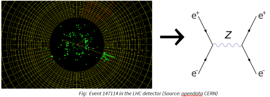
This is a figure of an event recorded from Compact Muon Solenoid(CMS) detector of Large Hadron Collider (LHC) used to extract the data of particles and record in the '.csv' file used below. Each track shown by a distinct line contains the information of various particles for example muon, electron, neutrino and photon tracks in the figure here later used to analyze different phenomena. The figure to the right of event is the Feynman diagram of the process where Z particle is the intermediate vector boson.
Importing the dataset:
Importing the dataset:
In[]:=
cern=CloudImport["https://www.wolframcloud.com/obj/Stoicishiv/dielectron.csv"]
Out[]=
Preprocessing
Preprocessing
Removing ‘Event’ and ‘Run’ column:
In[]:=
cernd=Drop[cern,0,2]
Out[]=
First two columns were just meant for the identity of the data included, hence removed.
Removing extra keywords:
In[]:=
cernd[All,KeyMap[Replace["px1 "->"px1"]]];
Identifying non-numerical data:
In[]:=
CountDistinct[Cases[cernd,{___,"nan"|"N/A",___}]]
Out[]=
85
Replacing non-numerical with the mean of the column it lies in:
In[]:=
filtercern=cernd/."nan"->Mean[cernd[[2;;200,17]]]
Out[]=
Extracting a numerical dataset:
In[]:=
filtercernd=filtercern[[2;;100001,All]];
Statistical summary of the dataset:
In[]:=
ResourceFunction["StatisticsSummary"][filtercernd]
Out[]=


This summary affirms the dataset we have preprocessed from ‘count’ and ‘non-numeric’ parameters of each column. Several more features are given in the table which gives an idea of the dataset.
Dataset Features
Dataset Features
◼
Energy
Plotting different features of energy for both the particles:
Energy of the particle 1 lies mostly below 50 GeV, but is distributed uniformly in the mass range. This is due to decay of the electrons in several light-particles.
Distribution of energies of both the particles are quite symmetrical.
◼
Momentum
Plotting different features of the momentum(x, y and z components) of particles and their combined scatter plot:
◼
Transverse momentum
Plotting transverse momentum of particles:
Transverse momentum is the resultant of momentum(x and y) components. The distribution gives the idea that momentum transfer between the beam and the particle is highest below 10 GeV.
◼
Pseudorapidity
Plotting pseudorapidity of the particles:
The graph of both the particles shows that particle 2 is less uniformly distributed around beam axis i. e. some are way too close and far than the particle 1. Particle 1 is uniformly distributed around the beam axis i. e. having almost same value of η.
◼
Charge
Visualizing the charge distribution of both particles:
This graph is amazingly symmetrical being exactly same distribution of charges giving an idea that electrons and anti-electrons are equal constituent of both particles 1 and 2.
◼
Mass
Plotting mass distribution with bin width set to 100:
It has a concentration on the minimum value of 2 and two further peaks can be observed.
◼
Numerical Features
Correlation matrix is the best way to observe the correlation between different coefficients of the data.
Plotting the correlation matrix of the dataset:
The parameters closely related are:
◼
E1(2) and pt1(2)
◼
phi1(2) and py1(2)
◼
eta1(2) and pz1(2)
◼
pt1(2) and M
Visualizing scatter plot of first three closely related set of parameters of both particles:
All the scatter plots verify the strong correlations between different coefficients. One having highest coefficient can easily be correlated linearly under regression.
Predicting the Invariant mass
Predicting the Invariant mass
In this section let’s use Mathematica’s machine learning functionalities and compare them for the task of predicting the invariant mass of electrons. First, we must reshape the data:
Shape the preprocessed data:
Split the data into a pair of shuffled training and testing sets using a Resource Function:
Define both the datasets:
Visualize a sample of dataset defined above:
Train a PredictorFunction using ‘Nearest Neighbor’ method:
Visualize the information of the PredictorFunction:
Evaluate the performance of the PredictorFunction using the test data:
Standard deviation is a measure of how dispersed the data is in relation to the mean. Low standard deviation means data are clustered around the mean, and high standard deviation indicates data are more spread out. The predictor measurement information indicated we have a very diverse predicted dataset.
Train PredictorFunction using different methods:
Notice that Linear Regression took the most time to train and got the higher standard deviation while Random Forest took the less time and got the smaller standard deviation(despite GradientBoostedTrees method)
Create a custom neural network using NetChain:
Train a custom neural network to predict the value of the invariant mass of electrons:
R-squared is a goodness-of-fit measure for regression models. R-squared measures the strength of the relationship between a model and the dependent variable on a convenient 0 – 1 scale with 1 representing a model that explains all the variation in the response variable around its mean.
The R-squared value of both Custom and Built-in Net are very close to 1 and this proves the Neural Network we trained and chosen(methods) in this project very accurately predict the Invariant mass of the dielectron.
The R-squared value of both Custom and Built-in Net are very close to 1 and this proves the Neural Network we trained and chosen(methods) in this project very accurately predict the Invariant mass of the dielectron.
Concluding remarks
Concluding remarks
We wanted to understand how a collision in high energy looks like. We chose collision of particles from Lepton family (in this project, electron.) We saw how Standard Model can be used to determine the basic features of the collision. We tried to understand the concept of ‘Invariant mass’ using different parameters of the collision. In our project we are trying to predict the ‘Invariant mass’ instead of just taking Mean of the Invariant mass dataset or calculating through the formula. The project carries out as follows:
1. The dataset has been imported and preprocessed.
2. Various features of the dataset have been analyzed randomly. Both particles had amazingly equal distribution of charges.
3. We analyzed the closeness between different parameters using correlation matrix and ‘scatter plotting’ them.
4. We then shaped the dataset and divided them for training and testing.
5. We deployed different methods for the PredictorFunction on the training dataset.
6. We then created a custom Neural Network using NetTrain and trained it to predict Invariant mass.
We checked for the R-squared value of the dataset trained by the ‘custom’ and ‘built-in’ Neural Network and Voilà it fits perfectly.
Particle physicists are constantly looking for more accurate tools for analyzing the collision and Machine Learning using Neural Network can be an optimum choice if it works perfectly in different processes like in our project.
Future Plans and Ideas
Future Plans and Ideas
Keywords
Keywords
◼
Collision
◼
LHC
◼
Invariant mass
◼
Machine learning
◼
Particle physics
◼
Neural Network
◼
Electron
◼
Data analysis
Acknowledgment
Acknowledgment
Mentor: Julián Laverde
Thanks to my mentor Julián Laverde for his immense help in the project and Mike for brainstorming in sorting out the physics part.
A big thanks to Rahul and other TA’s for bearing my stupid questions and codes.
Tuseeta and Mads for guiding throughout with their progress checks.
Last but not the least the fellow students of the School from whom I learned a lot.
References
References