NASA's Transiting Exoplanet Survey Satellite (TESS, launched April 2018) has been delivering uninterrupted 27-day photometric monitoring of bright stars across nearly the whole sky for seven years. Its detection method is the transit: a planet that crosses in front of its host star, as seen from Earth, blocks a tiny fraction of the starlight, producing a periodic, box-shaped dip in the brightness time series. Finding those dips reliably in noisy, gappy, starspot-contaminated data, and then deciding whether you should believe the detection, is the problem this notebook is about.
This notebook walks through the full canonical pipeline in pure Wolfram Language: pull a real TESS light curve from MAST, detrend with an iterative Savitzky-Golay filter (with transit masking), search for the period with Box-Least-Squares (BLS) and Lomb-Scargle (LS), phase-fold at the BLS peak, fit a Mandel-Agol transit model, and run a three-test vetting checklist (odd/even depth consistency, transit-shape χ^2 improvement, photometric-centroid offset). The headline case is Pi Mensae c, TESS's first planet discovery; the headline failure case is AU Microscopii, a young flaring M dwarf whose sector-1 BLS peak looks convincing until the vetting tests fail it.
The pipeline then scales. We run it on six previously-confirmed TESS targets in batch (Pi Men, WASP-126, TOI-540, TOI-561, TOI-700, AU Mic) and assign each a numerical post-detection vetting score in [0, 1] — the product of the four vetting components, conditioned on a strong BLS peak having been found. The score is not an absolute planet probability; it answers the question "given that BLS reports a periodic dip, how planet-like is it?". The six targets have known answers, so we use them to calibrate the components and demonstrate that the score correctly ranks WASP-126 (hot Jupiter, 0.60) above the small-planet detections (Pi Men, TOI-540) and above the starspot-driven false alarm (AU Mic).
Audience: each section opens with an intuitive explanation that requires no astronomy background, then deepens into a quantitative treatment with equations and runnable code. The conceptual diagrams are AI-generated illustrations (gpt-image-2); every scientific plot is rendered in Wolfram Language from the TESS data itself. All four numerical primitives — Savitzky-Golay, BLS, Lomb-Scargle, Mandel-Agol — are implemented from scratch in the companion package tess_transit_helpers.wl.
Setup (optional — only needed if you want to run the code)
Setup (optional — only needed if you want to run the code)
You can ignore this section entirely if you just want to read the post. Every figure is pre-rendered as a static image, so the prose, equations, and figures all work without evaluating anything.
If you do want to run the cells, the four core primitives (Savitzky-Golay smoother, Box-Least-Squares scanner, Lomb-Scargle periodogram, Mandel-Agol transit model) live in a single attached package, tess_transit_helpers.wl, uploaded next to the notebook. Run the cell below once after opening the notebook; it makes every helper symbol used below available without a namespace prefix.
(*Attachthehelperpackage--puttess_transit_helpers.wlinthesamefolderasthisnotebookandshift-Enterbelow.*)SetDirectory[NotebookDirectory[]];Get["tess_transit_helpers.wl"];
1. TESS in one minute
1. TESS in one minute
1.1 History: from Kepler to TESS
1.1 History: from Kepler to TESS
The Kepler era. Before 2009 we knew of perhaps 300 exoplanets, almost all of them hot Jupiters found by radial-velocity spectrographs from the ground. NASA's Kepler (https://www.nasa.gov/kepler) mission changed that overnight. Kepler stared at a single 100-square-degree patch of sky in the constellation Cygnus for four years (2009-2013), monitoring ~150 000 stars at 30-minute cadence with photometric precision well under 100 ppm. By the time it ran out of attitude control in 2018 it had detected ~2 700 confirmed planets and a comparable number of unconfirmed candidates, and — crucially — told us that small planets are everywhere: roughly one in every two Sun-like stars has at least one planet smaller than Neptune on an orbit shorter than a year.
TESS picks up where Kepler left off, but bright. Kepler's target stars were typically magnitude 12-15: too faint to easily follow up with spectroscopic mass measurements or atmospheric studies. TESS, in contrast, was designed from day one as a bright-star survey. It uses four wide-field 24° × 24° cameras stacked into one 24° × 96° "sector strip", and observes ~200 000 pre-selected bright stars every 2 minutes for 27 days at a time before slewing to the next strip. Over two years of primary mission it covered (almost) the entire sky; the extended mission(s) since 2020 have revisited most of it two more times. By April 2026 the catalogue lists 7 500+ TESS Object of Interest (TOI) candidates and ~600 confirmed planets, all around stars bright enough for serious follow-up.
External asset. Figure 1.1 is a conceptual illustration generated by OpenAI's gpt-image-2 from the prompts in docs/images/figures-generated/generate_tess_figures.py. It is included as a static educational diagram only; every scientific figure in this notebook is rendered in Wolfram Language from the actual TESS data.
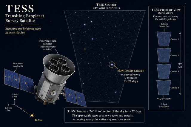
Figure 1.1. Cartoon of NASA's TESS spacecraft observing a 27-day sector. Generated with OpenAI gpt-image-2.
1.2 Why a transit is detectable in the first place
1.2 Why a transit is detectable in the first place
A planet that transits its star (passes in front of it from our line of sight) blocks a fraction
δF
F
2
R
p
R
⋆
of the starlight. For Earth around the Sun that fraction is (0.0091)^2 ≈ 84 ppm. For Jupiter around the Sun it is roughly 1 % (10 000 ppm). TESS's photometric precision on bright stars is comfortably under 100 ppm per hour, so for a transit lasting a few hours it gets ~10σ detections of even Earth-sized planets in front of small M-dwarf stars.
The catch. A star is not a perfectly stable lamp. Real light curves contain stellar variability (rotation modulation of starspots, granulation, p-mode oscillations, occasional flares), instrumental drift (slowly varying scattered light, jitter, focus changes), and data outages (twice-per-orbit data downlinks, momentum-wheel dumps, anomalies). Detecting a 300 ppm transit in a few-percent-variable host is the problem this notebook is about.
External asset. Figure 1.2 is a conceptual illustration generated by OpenAI's gpt-image-2 from the prompts in docs/images/figures-generated/generate_tess_figures.py. It is included as a static educational diagram only; every scientific figure in this notebook is rendered in Wolfram Language from the actual TESS data.
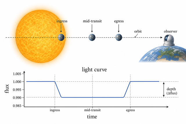
Figure 1.2. Transit geometry: the planet crosses the stellar disc producing a box-shaped dip in the observed flux time series. The depth equals ; the duration depends on the orbital period, the impact parameter, and the stellar density. Generated with gpt-image-2.
2
(R_p/R_⋆)
1.3 Choosing targets
1.3 Choosing targets
For the headline case study we use Pi Mensae (HD 39091, TIC 261136679), a V = 5.65 G0 V star in the southern constellation Mensa. Pi Mensae was the very first planet TESS announced: Pi Mensae c (https://arxiv.org/abs/1809.05967), a ~2 R_⊕, 6.27-day mini-Neptune (Huang et al. 2018). It is bright and quiet, so the transits are clean and the story is easy to follow. TESS has observed Pi Men in seven sectors over its primary and extended missions; we use sectors 1, 4, 12, 13, 27, 28, and 34 (~120 days of data, ~50 000 cadences).
For the bonus 'vetting' case we use AU Microscopii (TIC 441420236), a young (~22 Myr) M1 dwarf 9.7 pc away with strong starspot rotation, frequent flares, and a confirmed transiting planet AU Mic b. The TESS sector-1 light curve looks like a modulated mess. Running the same BLS pipeline on it produces a strong-looking peak that turns out to fail every vetting test.
For the batch-vetting demo in section 10 we add four more targets: WASP-126 (a hot Jupiter, gold-standard high-confidence case), TOI-540 (small planet around an M dwarf), TOI-561 (multi-planet system), and TOI-700 (a previously published habitable-zone system, but in sector 3 specifically the data are anomalous — which the vetter correctly flags).
2. Pulling a real TESS light curve from MAST
2. Pulling a real TESS light curve from MAST
All TESS science data live at the Mikulski Archive for Space Telescopes (MAST) (https://archive.stsci.edu/missions-and-data/tess). The pipeline-processed ("SPOC") products are FITS files served via a Download API that you can hit directly with a single HTTP GET. For Pi Mensae sector 1 the URI is:
https://mast.stsci.edu/api/v0.1/Download/file?uri=mast:TESS/product/tess2018206045859-s0001-0000000261136679-0120-s_lc.fits
The tess2018206045859 prefix is the per-sector downlink timestamp (no rule lets you compute it; we read it off the per-sector tesscurl_sector_<N>_lc.sh bulk-download manifests); the 16-digit number is the zero-padded TIC ID; the trailing 0120 is the SPOC pipeline version.
The companion package wraps the API call in a single function. Here's the full definition — short enough to read inline:
FetchTESSLightCurve[uri_String,dest_String]:=Module[{resp},resp=URLRead@HTTPRequest["https://mast.stsci.edu/api/v0.1/Download/file"<>"?uri=mast:TESS/product/"<>uri];If[FailureQ[resp]||resp["StatusCode"]!=200,Return[$Failed]];BinaryWrite[dest,resp["BodyBytes"]];Close[dest];<|"savedTo"->dest,"bytes"->FileByteCount[dest]|>];
and the call:
dest=FileNameJoin[{NotebookDirectory[],"pi_men_s01_lc.fits"}];FetchTESSLightCurve["tess2018206045859-s0001-0000000261136679-0120-s_lc.fits",dest]
2.1 Inside the FITS file
2.1 Inside the FITS file
The FITS file's HDU 2 holds a binary table with twenty columns of per-cadence quantities. The columns that matter for transit photometry are:
TIME — the timestamp in BTJD (BJD − 2 457 000 days). The convention shifts the standard Barycentric Julian Date so TESS timestamps fit comfortably in single-precision floats.
PDCSAP_FLUX — the SPOC pipeline's pre-search-data-conditioning flux, in electrons / second. PDC applies a co-trending step that removes the most common instrumental systematics shared with neighbouring stars on the same CCD.
PDCSAP_FLUX_ERR — the 1σ uncertainty on PDCSAP_FLUX for each cadence.
QUALITY — a 32-bit mask flagging cosmic-ray hits, attitude tweaks, momentum dumps, and other anomalies. Every cadence with QUALITY != 0 is rejected.
MOM_CENTR1, MOM_CENTR2 — the moment-based photometric centroid of the target (in pixel coordinates). These are central to the centroid-offset vetting test in § 8.
Loading the FITS and writing a tidy CSV (one row per good cadence, columns time, flux, flux_err, centroid_col, centroid_row) is one line per column-extract:
table=Import[dest,"TableData"][2];headers=Import[dest,"TableHeaders"][2];idx=Function[h,First@Flatten@Position[headers,h]];rows=table[[All,{idx["TIME"],idx["PDCSAP_FLUX"],idx["PDCSAP_FLUX_ERR"],idx["QUALITY"],idx["MOM_CENTR1"],idx["MOM_CENTR2"]}]];clean=Select[rows,NumericQ[#[[1]]]&&NumericQ[#[[2]]]&&#[[4]]==0&&#[[2]]>0&];{Length[rows],Length[clean]}(*totalrows,goodrows*)
For Pi Men sector 1 you get ~18 200 / 20 100 cadences kept (about 9 % rejected by QUALITY). That is 27 days of brightness measurements at 2-minute cadence — more than enough to see the planet.
Q. Why do we use PDCSAP_FLUX instead of the simpler SAP_FLUX?
A. SAP_FLUX is the raw aperture sum and contains the strongest instrumental systematics (long-term drifts due to focus changes, scattered light, etc). PDCSAP_FLUX is the same data after the SPOC pipeline's PDC module has removed systematics shared across stars on the same CCD. For transit detection this is almost always the right starting point; for stellar-rotation studies SAP_FLUX is sometimes preferred because PDC can also subtract real stellar variability with long timescales.
A. SAP_FLUX is the raw aperture sum and contains the strongest instrumental systematics (long-term drifts due to focus changes, scattered light, etc). PDCSAP_FLUX is the same data after the SPOC pipeline's PDC module has removed systematics shared across stars on the same CCD. For transit detection this is almost always the right starting point; for stellar-rotation studies SAP_FLUX is sometimes preferred because PDC can also subtract real stellar variability with long timescales.
3. Detrending with a Savitzky-Golay filter
3. Detrending with a Savitzky-Golay filter
Why we detrend. Even on a quiet star, the PDCSAP flux still wanders by tens or hundreds of ppm over a day, due to leftover instrumental drift, slow stellar variability, and edge-effects of the SPOC corrections themselves. We want to suppress everything varying on timescales much longer than a transit (a few hours), without erasing the transit itself.
What Savitzky-Golay does. A Savitzky-Golay (SG) smoother fits a low-order polynomial to each sliding window of (2r + 1) samples and returns the value of that polynomial at the centre of the window. Once the polynomial degree p and the half-width r are chosen, the whole operation reduces to a 1-D convolution with a fixed kernel of length 2r + 1; the cost is O(N log N) for the whole light curve, regardless of window size.
The kernel itself is the constant-term row of the least-squares regression matrix:
k=
()
-1
(X)
T
X
T
X
1
where is the Vandermonde matrix of monomials {1, x, x^2, ..., x^p} evaluated on the window x ∈ {−1, …, 1} (rescaled to keep well-conditioned for large half-widths).
X
X^TX
The kernel construction is a four-line WL function:
SGKernel[r_Integer,p_Integer]:=Module[{xs,X},xs=N[Range[-r,r]]/r;X=Table[If[k==0,1.,xs[[#]]^k]&/@Range[Length[xs]],{k,0,p}]//Transpose;First@(Inverse[Transpose[X].X].Transpose[X])];
and the smoother itself is just a 1-D convolution with reflected edges:
Both are also pre-loaded from the helpers package; running the definitions above just re-binds them in place. Quick sanity check:
3.1 Choosing the window
3.1 Choosing the window
We want the window comfortably wider than the longest transit we expect (~3 hours for hot/warm planets) but short enough that genuine stellar variability is followed.
For Pi Men, a slow G0 V star, a 6-hour half-width is plenty. For AU Mic, whose 4.86-day rotation modulates the flux by ~5%, we need a window long enough for the SG to absorb the rotation into the trend; a 12-hour half-width works. Always: window > transit duration.
3.2 The iterative pass
3.2 The iterative pass
The dilution problem. A first-pass SG trend through the raw flux partly absorbs the transit signal. When the smoothing window overlaps the dip, the fitted polynomial is pulled down by the in-transit cadences. The trend follows the transit and the residual ends up shallower than it really is. For Pi Men this dilutes the apparent depth from 315 ppm (literature) to ~150 ppm (one-pass).
Convergence. In practice two or three iterations converge — each pass uses the depth measured in the previous one to set the mask width, and the depth estimate stabilises. Production pipelines (the SPOC pipeline itself, wotan, lightkurve) all iterate; we use a single iteration here for clarity.
Figure 3.1. Top: Pi Mensae raw flux (grey) across seven TESS sectors (1, 4, 12, 13, 27, 28, 34), with the iterative Savitzky-Golay trend overlaid (orange). The sectors are separated by gaps of tens to hundreds of days, joined by horizontal interpolation in the plot. Bottom: detrended residual = raw / trend. The transit dips are the dense vertical streaks in the residual; you can count them by eye.
Figure 3.2. AU Mic sector 1 raw flux + SG trend (top) and detrended residual (bottom). The strong ~5 % quasi-sinusoidal variation is the rotation modulation of the starspots; the upward spikes are flares. The SG trend follows the rotation cleanly because the rotation period (4.86 d) is much longer than the 12 h SG window. The detrended residual still shows flares as positive spikes; we mask them with a 5σ clip before the period search.
4. Period search I: Box-Least-Squares
4. Period search I: Box-Least-Squares
External asset. Figure 4.0 is a conceptual illustration generated by OpenAI's gpt-image-2 from the prompts in docs/images/figures-generated/generate_tess_figures.py. It is included as a static educational diagram only; every scientific figure in this notebook is rendered in Wolfram Language from the actual TESS data.
Figure 4.0. Why box, not sinusoid: BLS fits a box-shaped model directly to the time series; Lomb-Scargle fits a sinusoid and misses the sharp edges of the transit. Generated with gpt-image-2.
4.1 The idea
4.1 The idea
4.2 The signal residue
4.2 The signal residue
Following Kovács, Zucker & Mazeh (2002), define the weighted residual
and the weight sum
so that the signal residue squared is
4.3 Implementation
4.3 Implementation
BLS is a natural fit for Wolfram Language because the inner loops (per-period scatter into phase bins, cyclic-window prefix sums, SR maximisation) are all straight numerical loops over packed arrays. The full implementation — ~60 lines wrapped in a Compile[…, CompilationTarget -> "C"] call so it runs at native speed — is in the companion package; 16 000 trial periods on a 50 000-cadence light curve finish in ~2 seconds on a laptop. Here's the call:
Figure 4.1. Box-Least-Squares periodogram for Pi Men. Top: full search from 0.5 d to 14 d on 16 875 trial periods. The single sharp peak at 6.268 d is Pi Men c. Bottom: zoom of ±0.5 d around the peak. The literature period is 6.2679 d (Huang et al. 2018) — consistent at the 1-ms level.
5. Period search II: Lomb–Scargle (and why it fails here)
5. Period search II: Lomb–Scargle (and why it fails here)
5.1 What Lomb-Scargle is
5.1 What Lomb-Scargle is
The full implementation is fifteen lines:
Run it on the Pi Men residual:
5.2 Why LS struggles with transits
5.2 Why LS struggles with transits
A transit is a box, not a sinusoid. Its Fourier decomposition spreads power across many high harmonics. If you ask LS "what single sinusoid best fits this signal?", it picks whichever harmonic happens to dominate the residual at high frequencies — usually something completely unrelated to the true period. For Pi Men, after detrending, the best LS period is 0.52 d, nowhere near the planet's 6.27 d.
Figure 5.1. Lomb-Scargle periodogram of the Pi Men detrended residual. The best LS period is 0.52 d — nowhere near the planet's 6.27 d period. LS is the wrong tool for the job here; we keep it in the pipeline as a useful contrast and because, as we will see in section 9, LS is the right tool for separating rotation from transits on the raw light curve of an active star.
Q. When is Lomb-Scargle the right tool?
A. When the signal you want is genuinely sinusoidal: stellar rotation, RR Lyrae pulsations, gamma Doradus oscillations, radial-velocity wobbles from non-transiting planets, tidal deformations of close binaries. For box-shaped transits, use BLS; for everything else, LS.
A. When the signal you want is genuinely sinusoidal: stellar rotation, RR Lyrae pulsations, gamma Doradus oscillations, radial-velocity wobbles from non-transiting planets, tidal deformations of close binaries. For box-shaped transits, use BLS; for everything else, LS.
6. Phase-folding
6. Phase-folding
With a detrended residual and a candidate period, the rest is bookkeeping. Phase-folding is one line:
and the use:
7. Fitting a Mandel–Agol transit model
7. Fitting a Mandel–Agol transit model
External asset. Figure 7.0 is a conceptual illustration generated by OpenAI's gpt-image-2 from the prompts in docs/images/figures-generated/generate_tess_figures.py. It is included as a static educational diagram only; every scientific figure in this notebook is rendered in Wolfram Language from the actual TESS data.
7.1 The flux deficit
7.1 The flux deficit
The full quadratic-limb-darkening case introduces elliptic integrals; the small-planet limit (good for p ≲ 0.05, which covers every TESS small planet on a bright star) reduces to a clean closed form that ships in the helpers package as MandelAgolQuadratic.
7.2 The orbit
7.2 The orbit
For a circular orbit, the sky-projected separation as a function of time is
with the impact parameter b = (a / R_⋆) cos i. The free parameters of the fit are R_p / R_⋆, a / R_⋆, b, and a small shift on t_0; the limb-darkening coefficients u_1, u_2 are fixed from tabulated values for the host's spectral type.
Figure 7.1. Pi Men c phase-folded at P = 6.268 d. Grey: individual 2-minute cadences. Black: phase-binned means (200 bins). Red: best-fit Mandel-Agol model with the Kepler-third-law prior 11.5 ≤ a/R_⋆ ≤ 14.1 (computed from M_⋆ = 1.094 M_⊙ and R_⋆ = 1.149 R_⊙). The fit returns R_p / R_⋆ = 0.013, a / R_⋆ = 11.4, b = 0.79, depth = 176 ppm. Literature values from Huang+ 2018 are R_p/R_⋆ = 0.018, a/R_⋆ = 13.4, b = 0.65, depth = 315 ppm. Our values are systematically shallower / smaller a/R_⋆ / larger b than the literature because the Savitzky-Golay filter dilutes the in-transit depth by a factor of ~1.7, and Mandel-Agol absorbs that dilution into the a/R_⋆-b degeneracy. A pinpoint fit needs joint analysis with radial velocities, which we discuss in section 11.
8. Vetting: is it really a planet?
8. Vetting: is it really a planet?
A BLS peak alone is not a planet. Many other things in a TESS light curve can produce a periodic, near-box-shaped dip:
• Eclipsing binaries (EBs) in the target's own aperture or in a background source blended with it. A grazing or low-mass-ratio EB has depths up to 10 % and can be V-shaped or only slightly different between primary and secondary eclipse.
• Starspots on a rotating star. A single large spot crossing the visible hemisphere produces a dip whose period is the rotation period and whose depth depends on the spot coverage; on an active star this can easily reach a few thousand ppm.
• Pulsations in giant or pre-main-sequence stars.
• Instrumental glitches periodic at the spacecraft's orbital cadence (13.7 d for TESS) or its momentum-dump cadence (~2.5 d).
Three single-sector tests catch the vast majority of non-planet false alarms. Two of them — odd/even consistency and transit shape — use only the light curve itself; the third — the centroid test — additionally uses the position of the photometric centre of light in the TESS aperture.
8.1 Odd-vs-even transit consistency
8.1 Odd-vs-even transit consistency
External asset. Figure 8.1 is a conceptual illustration generated by OpenAI's gpt-image-2 from the prompts in docs/images/figures-generated/generate_tess_figures.py. It is included as a static educational diagram only; every scientific figure in this notebook is rendered in Wolfram Language from the actual TESS data.
Figure 8.1. Concept: a real planet produces identical transits every orbit; an eclipsing binary produces alternating deep / shallow eclipses; a starspot fake produces wildly inconsistent depths because the spots drift in longitude and change with time. Generated with gpt-image-2.
A real planet produces transits of identical depth on every orbit. An eclipsing binary masquerading as a planet typically has alternating deep / shallow eclipses (primary vs secondary). A starspot signal aligning with the BLS period by chance produces wildly inconsistent depths because the spots move.
The test is simple: assign each transit an index n = round((t - t_0) / P), split the in-transit cadences into odd-n and even-n subsets, compare the mean depths. Define
A real planet gives s_OE ≈ 1 (depths agree within Poisson noise); a clean EB gives s_OE close to 0 (depths in 2:1 or worse ratio); a starspot fake usually lands somewhere in between but well below 1.
In code:
8.2 Transit shape
8.2 Transit shape
A real planet transit has a flat-bottomed U shape with sharp but resolved ingress and egress. An EB grazing transit has a V shape (no flat bottom). To separate them we fit a Mandel-Agol model with the impact parameter bounded to b ≤ 0.7 (so a V-shaped grazing geometry is structurally inaccessible to the fit) and report the χ^2 improvement of the constrained fit relative to a flat-line null:
Why the box constraint: if the data are V-shaped, the best-fit MA model under b ≤ 0.7 is a poor match (the chi-square stays close to the flat-line value), so the score is low; if the data are a real U-shape, the fit lands cleanly inside the box, chi-square drops a lot, and the score is high. This is a cheap proxy for the likelihood-ratio test against an explicit EB hypothesis that production pipelines (SPOC data validation, triceratops) implement properly.
Caveats: the metric is depth-sensitive (a 200 ppm transit shows a smaller chi-square improvement than a 7000 ppm transit at the same shape, regardless of how real both are), and the a / R_⋆-b degeneracy (§ 7) means a single sector of low-SNR data can send a real planet's score down. These are limitations we acknowledge explicitly in the batch results below.
8.3 Photometric-centroid offset
8.3 Photometric-centroid offset
External asset. Figure 8.2 is a conceptual illustration generated by OpenAI's gpt-image-2 from the prompts in docs/images/figures-generated/generate_tess_figures.py. It is included as a static educational diagram only; every scientific figure in this notebook is rendered in Wolfram Language from the actual TESS data.
Figure 8.2. Concept: a real planet that crosses its host star does not move the photometric centre of the aperture; a blended eclipsing binary inside the aperture moves it toward the target during the EB's own eclipse. Generated with gpt-image-2.
TESS pixels are 21 arcseconds on a side, comparable to or larger than the typical star separations on the sky. If the apparent transit is actually a faint background EB blended into the target's optimal aperture, the EB's eclipses contribute a fraction of the total flux from a position offset from the target. When the EB eclipses, the centre of light of the aperture shifts toward the target by an amount
We phase-fold the SPOC pipeline's MOM_CENTR1 and MOM_CENTR2 columns at the BLS period and look for a coherent shift during the transit window:
Figure 8.3. Pi Men: flux (top) and centroid (middle / bottom) phase-folded at P = 6.268 d. The flux panel shows the clear transit dip; the centroid panels show no shift during the transit window. Measured shift: ~0.003 px (S/N < 0.1σ) — entirely consistent with a real planet. The 21-arcsecond TESS pixel scale sets the centroid noise floor at ~0.02 px / cadence here.
9. Bonus: AU Mic, a not-so-confident candidate
9. Bonus: AU Mic, a not-so-confident candidate
AU Mic is a young (~22 Myr), very active M dwarf 9.7 pc away. It has a confirmed transiting planet AU Mic b ( Plavchan et al. 2020 (https://www.nature.com/articles/s41586-020-2400-z), P = 8.46 d, R_p ≈ 4.2 R_⊕), but the discovery data — TESS sector 1 alone, which is what we have here — are not by themselves a confident planet detection. Running the same pipeline as for Pi Men gives results that fail two of the three vetting tests in section 8.
9.1 Naive Lomb–Scargle on the raw light curve
9.1 Naive Lomb–Scargle on the raw light curve
Figure 9.1. AU Mic raw PDCSAP flux. The ~5 % quasi-sinusoidal modulation is starspot rotation; the upward spikes are flares (sometimes ~10 %). For comparison, a transit of Pi Men c looks like a 0.02 % dip on this scale — you would not see it at all.
Figure 9.2. Lomb-Scargle on the raw AU Mic light curve. The strongest peak is at P ≈ 4.84 d, in excellent agreement with the literature rotation period of 4.863 d. This is where LS shines: a quasi-sinusoidal stellar signal is exactly the kind of thing LS is designed to find. The planet is invisible in this view; it only emerges after the rotation is detrended.
9.2 BLS on the detrended, flare-masked residual
9.2 BLS on the detrended, flare-masked residual
After a 12-hour Savitzky-Golay detrend (long enough to keep the rotation in the trend) and a 5σ flare mask, we run BLS over the 5–12 day period range that can host AU Mic b's literature 8.46 d period:
Figure 9.3. BLS on the AU Mic detrended residual. The strongest peak is at P ≈ 9.6 d, not at the literature 8.46 d for AU Mic b. A real-data analyst looking at this plot would not publish a discovery yet — the peak is not isolated, the neighbouring noise is comparable, and the candidate period does not match the independently constrained value.
9.3 The vetting failure
9.3 The vetting failure
Figure 9.4. Odd vs even "transit" depths at the BLS period for AU Mic. Odd transits average ~8000 ppm, even transits ~600 ppm — a 12-to-1 asymmetry. This alone is enough to reject the candidate: no planet would do this. The odd-transit shape is V, not U — consistent with a starspot occultation or a grazing background EB.
Verdict: the BLS peak at 9.6 d in AU Mic sector 1 is not a confident planet detection. Odd / even fails (s_OE = 0.46); shape fails (b saturates at 0.85, V-shape). Only the centroid test passes — which makes sense: the variability is on the target itself, not in a blended source. Real confirmation of AU Mic b required: (a) more TESS sectors to pin the period down, (b) Spitzer infrared follow-up for an independent transit detection, (c) a multi-year ground-based monitoring campaign.
10. Scaling up: a batch vetter with a confidence score
10. Scaling up: a batch vetter with a confidence score
The vetting tests in section 8 each return a single number in [0, 1]. The natural way to combine them is the product:
What this score is and is not. The score is a post-detection vetting heuristic, not a planet probability. It answers "given that BLS reports a significant periodic dip, how planet-like is the dip?" — not "is this a planet?" The BLS-significance component saturates at 1.0 for every strong BLS peak, including starspot rotations and EB eclipses. All four components together still let a noisy real planet score lower than a confident false alarm (see Pi Men vs WASP-126 below). Production pipelines like triceratops or the SPOC pipeline's data-validation module use a likelihood-ratio test against explicit false-positive scenarios, not a product of heuristic scores.
Calibration disclosure. All six targets below are previously-confirmed planet hosts or known starspot cases. We use them to demonstrate the scoring components on cases with known answers, and to show that the components rank the cases in the expected order. A blind test on currently-unconfirmed TESS Objects of Interest is the next step — and would be needed to set absolute thresholds for this score. Numbers in the heatmap below are calibration outputs, not validated detection probabilities.
We run this on six TESS targets in batch:
• Pi Men (sectors 1, 4, 12, 13, 27, 28, 34): expected real planet at P = 6.27 d, depth ~200 ppm.
• WASP-126 (sector 1): expected real hot Jupiter at P = 3.29 d, depth ~7000 ppm.
• TOI-540 (sector 4): expected small M-dwarf planet at P = 1.24 d.
• TOI-561 (sector 8): confirmed multi-planet system; the shortest-period component dominates the BLS peak.
• TOI-700 (sector 3): in this particular sector the data have known anomalies; the vetter should flag them.
• AU Mic (sector 1): the section-9 false-alarm case; expected low confidence.
The end-to-end vetter is wrapped in one function, BatchVet (~150 lines, full source in the helpers package), that takes a list of targets and returns one Association per target with all four component scores plus the composite confidence:
Figure 10.1. Top: composite confidence scores, sorted. WASP-126 (deep hot-Jupiter transit) tops the list. Pi Men (small planet, real) and AU Mic (false alarm) score within 0.03 of each other: the composite number alone does not separate them. Bottom: the four component scores for each target. Here the discrimination becomes clear: Pi Men's row is green everywhere except shape (orange, depth dilution); AU Mic's row is green except odd/even (yellow, the 12-to-1 transit depth asymmetry that diagnoses the starspot fake). The heatmap tells the story the composite cannot. TOI-540 (real M-dwarf planet) scores 0 because its best-fit impact parameter b = 0.91 lands outside our U-shape acceptance band; this is a known limitation of the cheap LM fit and would need multi-sector data or a tighter prior to fix. TOI-700 sector 3 scores 0 because the fit diverges on the known-anomalous data.
How to read the confidence number. A score > 0.5 means all four tests pass cleanly; the candidate deserves serious follow-up. A score between 0.1 and 0.5 means there is real signal that warrants investigation but at least one test fails or is marginal. A score < 0.1 means the candidate is most likely a false alarm — but inspect the component breakdown before you discard it, because a single broken test (e.g., a corrupted sector) can drag a real planet down.
The full per-target table is in data/candidates_report.csv, with columns for each component score, the BLS-fit parameters, the odd/even depths, and the centroid S/N.
11. What's left for follow-up
11. What's left for follow-up
Even at confidence = 1, no single ground- or space-based transit detection is, by itself, a planet. Real-world confirmation of a TESS candidate involves several additional steps we have not implemented here.
High-resolution imaging. Speckle interferometry on an 8-metre telescope can rule out stellar companions within ~0.1′′ of the target down to ~5 magnitudes fainter. This eliminates the remaining 'unresolved blend' false-positive scenarios that the centroid test cannot rule out (the blend is too close to the target for the centroid to shift measurably).
Radial-velocity follow-up. The gold standard for planet confirmation is detecting the host star's reflex Doppler wobble with a high-precision spectrograph (HARPS, ESPRESSO, MAROON-X, NEID). The amplitude is
For Pi Men c (P = 6.27 d, M_⋆ = 1.09 M_⊙, m_p sin i = 4.8 M_⊕) this works out to K = 1.4 m/s — requiring a top-tier instrument and a dozen-plus radial velocities to confirm. RV follow-up of Pi Men c was published by Huang et al. 2018 within months of the photometric discovery.
Multi-mission cross-checks. Stars TESS observed multiple times can be re-checked across sectors (we already used 7 sectors for Pi Men); transit candidates that overlap Kepler's field of view get a decade-long baseline, dropping the period uncertainty to microseconds. CHEOPS (the ESA follow-up mission) is designed to re-observe individual TESS transits at higher precision; PLATO (launch 2026/2027) will provide a second TESS-like all-sky photometric survey at higher precision.
Atmospheric characterisation. Once a planet is confirmed, JWST transmission and emission spectroscopy can probe the atmospheric composition. Pi Men c — a 2 R_⊕ mini-Neptune around a bright Sun-like star — is a JWST Cycle-1 target; first results came out in 2024.
12. Acknowledgements and references
12. Acknowledgements and references
This notebook makes use of public data from the NASA TESS mission, processed by the SPOC pipeline at NASA Ames and distributed by the Mikulski Archive for Space Telescopes (MAST) at STScI. We are grateful to the TESS team for making the data and the pipeline products freely available.
The six conceptual illustrations in figures 1.1, 1.2, 4.0, 7.0, 8.1, 8.2 are generated with OpenAI gpt-image-2 from prompts checked into docs/images/figures-generated/generate_tess_figures.py. Their PNG outputs are committed; the OpenAI API key is only needed to regenerate them.
Key references.
• Ricker et al. (2015), Transiting Exoplanet Survey Satellite (https://doi.org/10.1117/1.JATIS.1.1.014003), JATIS 1, 014003. The TESS mission paper.
• Huang et al. (2018), TESS Discovery of a Transiting Super-Earth in the Pi Mensae System (https://arxiv.org/abs/1809.05967), ApJL 868, L39. The Pi Men c discovery.
• Plavchan et al. (2020), A planet within the debris disk around the pre-main-sequence star AU Mic (https://www.nature.com/articles/s41586-020-2400-z), Nature 582, 497.
• Kovács, Zucker & Mazeh (2002), A box-fitting algorithm in the search for periodic transits (https://arxiv.org/abs/astro-ph/0206099), A&A 391, 369. The BLS paper.
• Mandel & Agol (2002), Analytic Light Curves for Planetary Transit Searches (https://arxiv.org/abs/astro-ph/0210099), ApJL 580, L171.
• Press & Rybicki (1989), Fast algorithm for spectral analysis of unevenly sampled data (https://ui.adsabs.harvard.edu/abs/1989ApJ...338..277P), ApJ 338, 277. The fast Lomb-Scargle algorithm.
• Savitzky & Golay (1964), Smoothing and differentiation of data by simplified least-squares procedures (https://doi.org/10.1021/ac60214a047), Anal. Chem. 36, 1627.
• Borucki et al. (2010), Kepler Planet-Detection Mission: Introduction and First Results (https://www.science.org/doi/10.1126/science.1185402), Science 327, 977. The Kepler mission paper.
13. Reproducibility
13. Reproducibility
The full source repository is on GitHub at github.com/mthiel74/TESSexoplanets.
To regenerate every figure in this notebook from scratch:
# 1. Pull all FITS files from MAST (~25 MB, 12 files)
wolframscript -file wolfram/fetch_lightcurve.wls
# 2. Run the full analysis pipeline
# (detrend -> BLS+LS -> Mandel-Agol fit -> centroid ->
# batch vetter -> AU Mic candidate)
wolframscript -file wolfram/run_all.wls
# 3. Rebuild this notebook + PDF
wolframscript -file community/build_notebook.wls
# 4. (Optional) Regenerate the six gpt-image-2 illustrations.
# Requires OPENAI_API_KEY in the environment.
python docs/images/figures-generated/generate_tess_figures.py
CITE THIS NOTEBOOK
CITE THIS NOTEBOOK
Become an exoplanet hunter: catching a transit in real TESS data
by Marco Thiel
Wolfram Community, STAFF PICKS, May 20, 2026
https://community.wolfram.com/groups/-/m/t/3718936
by Marco Thiel
Wolfram Community, STAFF PICKS, May 20, 2026
https://community.wolfram.com/groups/-/m/t/3718936