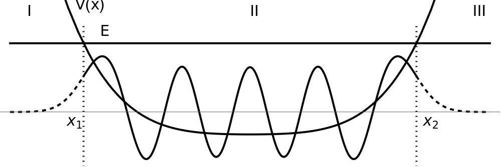
Fixing Fig. 2.5 from MQM2e (WKB Schematic)
Fixing Fig. 2.5 from MQM2e (WKB Schematic)
This follows the Featured Example called “Eigenproblems”
This follows the Featured Example called “Eigenproblems”
In[]:=
Remove["Global`*"]
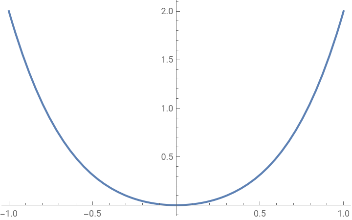
First come up with a potential to solve. Make it symmetric to make it easy
In[]:=
v=x^2+x^4;Plot[v,{x,-1,1}]
Out[]=
Now solve the eigenvalue equation
In[]:=
pfun=ParametricNDSolveValue[{-u''[x]+vu[x]ϵu[x],u[0]1,u'[0]0},u,{x,-10,10},{ϵ}];
In[]:=
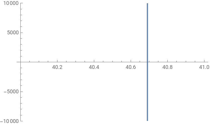
Plot[pfun[ϵ][9],{ϵ,40,41},PlotRange{-10^4,10^4}]
Out[]=
In[]:=
ϵVal=ϵ/.FindRoot[pfun[ϵ][9],{ϵ,40}]

Out[]=
40.6904
Find the classical turning points
In[]:=
xCTP=x/.Solve[v==ϵVal,x][[4]]
Out[]=
2.42868
Make the plot
In[]:=
vTrans[e_]=0.05e-1/2;func=pfun[ϵVal][x];lims=3.5;Show[Plot[vTrans[v],{x,-lims,lims},PlotRange{-1.2,2.5},PlotStyle{Black,Thick},Axes{True,False},TicksNone,AxesStyleThin,AspectRatio1/3,ImageSize500],Plot[vTrans[ϵVal],{x,-lims,lims},PlotStyle{Black,Thick}],Plot[func,{x,-xCTP,xCTP},PlotStyle{Black,Thick}],Plot[func,{x,-lims,-xCTP},PlotStyle{Black,Dashed}],Plot[func,{x,xCTP,lims},PlotStyle{Black,Dashed}],ListLinePlot[{{xCTP,-2},{xCTP,2}},PlotStyle{Black,Dotted}],ListLinePlot[{{-xCTP,-2},{-xCTP,2}},PlotStyle{Black,Dotted}],Graphics[Text[Style["I",FontSize15],{-3.25,2.25},{-1,0}]],Graphics[Text[Style["II",FontSize15],{0,2.25},{-1,0}]],Graphics[Text[Style["III",FontSize15],{3.25,2.25},{-1,0}]],Graphics[Text[Style[Subscript[x,1],FontSize15],{-1.1xCTP,-0.2},{-1,0}]],Graphics[Text[Style[Subscript[x,2],FontSize15],{1.04xCTP,-0.2},{-1,0}]],Graphics[Text[Style["E",FontSize15],{-0.9xCTP,1.8},{-1,0}]],Graphics[Text[Style["V(x)",FontSize15],{-1.05xCTP,2.4},{-1,0}]]]
Out[]=