CITE THIS NOTEBOOK: Simulating state-vectors and density matrices with QuESTlink by Tyson Jones. Wolfram Community NOV 3 2022.
ORIGINAL ARTICLE: Jones, Tyson, and Simon Benjamin. QuESTlink?Mathematica embiggened by a hardware-optimised quantum emulator. Quantum Science and Technology, 5: 034012 (2020). https://doi.org/10.1088/2058-9565/ab8506.
See related discussion: Simulating Quantum Computers with QuESTlink
ORIGINAL ARTICLE: Jones, Tyson, and Simon Benjamin. QuESTlink?Mathematica embiggened by a hardware-optimised quantum emulator. Quantum Science and Technology, 5: 034012 (2020). https://doi.org/10.1088/2058-9565/ab8506.
See related discussion: Simulating Quantum Computers with QuESTlink
QuESTlink is a symbolic and numerical simulator of quantum circuits, state-vectors, density matrices and Hamiltonians, which aims to be as usable as it is fast. It supports multithreading, GPU-acceleration and deployment to remote hardware, and a wide array of simulation, drawing and analysis facilities.
Installation
Installation
Downloading, installing and configuring a quantum simulator can be a tedious overhead to jumping into research questions. We make obtaining the latest QuESTlink version a breeze:
Import["https://qtechtheory.org/questlink.m"];CreateDownloadedQuESTEnv[];
Demonstrations
Demonstrations
Circuits are specified symbolically in a concise syntax faithful to the quantum computing literature.
c=Circuit[][[θ]][ϕ]R[λ,];DrawCircuit[c]
H
0
H
1
H
2
H
3
S
1
T
3
C
0
X
3
SWAP
2,3
C
2,0
Ry
1
Rz
3
X
0
Z
2
Y
3
They can be analytically studied
m=CalcCircuitMatrix[c];m〚1,1〛
1
4
-
ϕ
2
λ
2
1
4
π
4
ϕ
2
λ
2
or efficiently numerically simulated in the QuEST C++ backend, which one can compile to be multithreaded, GPU-accelerated and server-side.
ψ=CreateQureg[4];ApplyCircuitψ,c/.θ,ϕ,λ;GetQuregMatrix[ψ]//MatrixForm
π
3
π
4
π
5
0.190101-0.162362 |
0.148292+0.0614245 |
0.162362+0.190101 |
-0.0614245+0.148292 |
0.296259+0.0809047 |
0.174306-0.117257 |
-0.0809047+0.296259 |
0.117257+0.174306 |
0.291039+0.120552 |
0.162362+0.190101 |
-0.120552+0.291039 |
-0.190101+0.162362 |
0.043959+0.280955 |
0.164356-0.0605984 |
-0.280955+0.043959 |
0.0605984+0.164356 |
This allows advanced questions to be rapidly answered, such as the approximate energy extrema of our circuit with equal parameters under a funky Pauli Hamiltonian:
h=SimplifyPaulis + .2(+++)//Chop
3
(.1+.2)
X
0
Z
0
X
1
2
(.1-.6+.5)
X
0
Y
1
Z
2
Z
3
Y
0
Y
1
Z
2
X
3
X
2
X
3
Y
3
Y
0
Z
0
Z
1
X
1
X
2
-0.00186+0.2+0.2+0.2+0.0062+0.2+0.00036-0.0012
X
0
X
1
X
2
X
2
X
3
Y
0
Y
3
X
1
Z
0
Z
0
Z
1
Y
1
Z
2
Z
3
Y
0
Z
1
Z
2
Z
3
tmp=CreateQureg[4];data=Table ApplyCircuit[InitZeroState[ψ],c/.{θv,ϕv,λv}]; CalcExpecPauliSum[ψ,h,tmp], {v,0,30,.1};ListLinePlot[data]{Max[data],Min[data]}
{0.142713,-0.173802}
Suzuki-Trotter simulation
Suzuki-Trotter simulation
Many quantum algorithms become trivial and concise to express. Here are all orders of the Suzuki-Trotter decomposition of a Hamiltonian h!
symmetrize[h_,λ_,1]:=λhsymmetrize[h_,λ_,2]:=With {s1=symmetrize[h,λ/2,1]}, Join[s1,Reverse[s1]]symmetrize[h_,λ_,n_?EvenQ]:=Block γ,p=1(4-),With{s=symmetrize[h,γ,n-2]},With{r=s/.γλp}, Join[r,r,s/.γ(1-4p)λ,r,r]gateify[Verbatim[Times][θ_,σ__]]:= R[2θ,Times[σ]]trotterize[h_,n_,r_,t_]:=With {s=symmetrize[List@@h,t/r,n]}, gateify/@Flatten@ConstantArray[s,r]
1/(n-1)
4
We have many ways to rapidly visualise these circuits.
DrawCircuit@trotterize[h,1,1,.1]
DrawCircuit@trotterize[h,2,1,.1]
CalcCircuitMatrix@trotterize[h,1,1,1]//MatrixForm
DrawCircuitTopology@trotterize[h,2,1,.1]
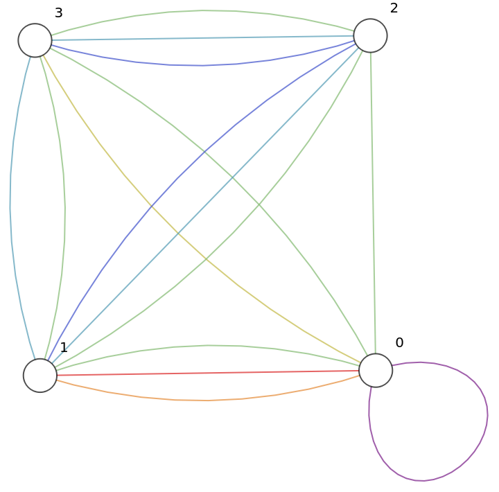


Let’s initialise a new qureg ψtrue to a future state prescribed directly by the Schrodinger equation
and compare it to the states produced by our Trotter circuits
Noisy simulation
Noisy simulation
Since we can modify our circuits symbolically, injecting noise into our circuits is easy!
We can numerically simulate these noisy circuits using density matrices.
Here is that noisiest order-6 Trotter state:
Hungry for more?
Hungry for more?