This notebook series is designed to introduce selected dynamic economic models to both advanced undergraduate and graduate students. Economists have relied on a series of economic models to better understand the otherwise highly complex causal relationship among many economic variables. Dynamic economic models set up by systems of either difference or differential equations are particularly useful in tracing the change in the quantity of unknown economic variables (e.g., the capital stock, demand for labor, aggregate output, etc.) and their interactions over time.
This notebook series aims to help students better understand the depth, usefulness, and limitations of major existing micro and macroeconomic models by demonstrating how we can use Wolfram Mathematica to replicate and reconstruct the core ideas and find dynamic solution of the model.
The model introduced in this notebook series include, among others, (1) the cobweb model of the quantity and price adjustment, (2) Keynes’s aggregate demand model, (3) Hicks’s ISLM model, (4) Samuelson’s investment accelerator model, (5) Kalecki’s investment delay model, (6) the predator-prey interaction model, (7) the epidemic model, (8) Ricardo’s three dimensional business cycle model, (9) Marx-Goodwin business cycle and growth model, (10) Smith’s and Ricardo’s growth model, (11) the Harrod-Domar growth model, (12) the Solow growth model, (13) the RBC model, (14) Romer’s new growth model, and (15) the circuit of capital model.
Introduction
Introduction
In the previous sessions, we have learned that Solow’s aggregate production function fails to explain how the so-called production technology evolves. We also learned that the RBC theorists modified the evolution of the production technology by introducing a random variation term without explaining how and where this source of variation comes from.
Paul Romer suggested slightly different ideas when explaining the change in the production technology. Instead of assuming that this production technology or the stock of knowledge is either growing at a constant rate or disturbed by random shocks, Romer explores the possibility that the invention and application of new stock of knowledge is an outcome of business firms’ deliberate efforts and resource allocation to their R&D sector (Romer 1990).
Romer’s growth model building strategy evolved over time. In his earlier paper, Romer focused on the possible increasing returns to scale property of the production technology and its unintentional spillover in the economy. He argued that a firm-specific production technology and/or the know-how can spread to other firms, thereby generating positive externality in the economy as a whole, even though the individual firm may experience diminishing returns to scale on its existing physical capital stock. In this formulation, Romer assumes that the individual firm’s production technology is non-excludable and non-diminishable by nature. Other firms do not incur substantial cost when obtaining this stock of knowledge because of this public good nature of production technology. As a result, the aggregate economy experiences increasing returns, rather than diminishing returns to scale (Romer 1986).
In his subsequent paper, Romer introduces the idea that the production technology can be an outcome of the firm’s deliberate efforts to invent and apply it in its final goods production activity. The representative firm in this new model makes a careful decision about how to allocate both the capital stock and labor input to its R&D sector, while engaging in the final goods production activity. With this new formulation, the firm-specific ‘know-how’ is no longer an accidental byproduct of utilizing the existing physical capital stock, which could be spread and obtained by other competing firms. Instead, the firm’s stock of knowledge becomes partially excludable and non-rival in nature. Therefore, depending of the firm’s efficiency in allocating resources and the outcome of its R&D sector, the firm’s final goods production is also affected (Romer 1990).
Since its inception, Romer’s model renewed the interest in economic growth and growth modeling, and it has been often called and classified as one variant of ‘new’ or ‘endogenous’ growth models. Following David Romer (2011) and Raghavendra and Piiroinen (2023)’s presentation, this note reconstructs Romer’s new growth model. For an analytical purpose, this notebook (1) presents an analytical system of two nonlinear differential equations that describe the production of both final goods and the stock of knowledge and (2) builds and creates two interactive charts that show the firm’s allocation decision and its effect on both the production of both final goods and the stock of knowledge. In the appendix, we also attempt to introduce a stochastic variation term inside the production of the stock of knowledge in the Romer model.
Aggregate production function and the growth of the capital stock
Aggregate production function and the growth of the capital stock
Just as his predecessors, Romer starts with the aggregate production function. Aggregate output is a function of the technology-augmented capital stock, in which the capital stock grows as a function of a constant average saving rate, the growth rate of labor force, and the given depreciation rate of the existing capital stock .
Y(t)=AK(t)
(
1
)
K
(
2
)where Y is output, K is the productive capital stock, A is an index of the production technology (or the stock of knowledge), s is the saving rate, n is the growth rate of labor force, and δ is a constant depreciation rate.
Substituting (1) into (2) and dividing every term by K(t):
K
K(t)
K
(
3
)The growth rate of the capital stock becomes a positive function of the knowledge stock A, given the constant savings, labor force, and the depreciation rate. How can we introduce and explain the change in A over time in this formulation?
Aggregate production function and the growth of the stock of knowledge
Aggregate production function and the growth of the stock of knowledge
Suppose that the economy consists of two sectors, or the representative firm has the following two sub-sectors: The first sector is where final consumption goods are produced and the other where the stock of knowledge, A, is invented. Let us call the latter the (R&D) sector. The representative firm makes a decision about how to allocate two factors of production (both the capital stock and labor input) into these two sectors.
If (0≤ ≤ 1) is the portion of labor input that is devoted to the R&D, the residual proportion 1 - will be the remaining labor input allocated to the final goods producing sector. Similarly, if we define (0≤ ≤ 1) as the unit of the existing capital stock that is devoted to the R&D sector, then the remaining capital stock, 1 - , must be allocated to the final consumption goods producing sector.
a
L
a
L
a
L
a
K
a
K
a
K
If the relative intensity of the capital stock used in the final goods production sector, α, is given under the constant returns to scale property assumption made about the production technology, the production function in the final goods producing sector can be represented by the following Cobb-Douglas production function:
Y(t)[A(t)(1-)L(t)],0≤α≤1
1-α
α
=[(1-)K(t)]
a
K
a
L
(
4
)Similarly, the growth of the stock of knowledge in the R&D sector is defined as:
A
β
(K(t))
a
K
γ
(L(t))
a
L
θ
(t)
(
5
)where B, β and γ are exogenously given constants. This knowledge production function expressed in terms of the growth rate form does not necessarily have constant returns to scale property in relation to both of the input, capital and labor. Therefore, the two exponents, β and γ does not necessarily add up to one (1). That is, β + γ ≠ 1. The parameter θ captures the effect of the existing stock of knowledge on the invention of new knowledge stock, or on the output of the R&D sector, and there is no restriction imposed on this parameter, too. That is, θ can be either positive or negative (θ > 0 or θ < 0).
The growth of labor input and the saving-investment causality
The growth of labor input and the saving-investment causality
Similar to the Solow growth models, suppose that labor force grows at a constant rate n, so that:
L
(
6
)We also assume that the average saving rate s is an exogenously given constant, and the saving drives investment. If we ignore the depreciation of the capital stock, for the moment, the capital stock accumulation can be expressed as:
K
(
7
)The derivation of the system of two differential equations
The derivation of the system of two differential equations
If we substitute (4) into (7) and divide by K(t), we get the following growth rate of the capital stock:
g
K
K
K(t)
α
(1-)
a
K
1-α
(1-)
a
L
1-α
A(t)L(t)
K(t)
(
8
)Similarly, if we divide (5) by A(t) to get the growth rate of the stock of knowledge:
g
A
A
A(t)
β
(K(t))
a
K
γ
(L(t))
a
L
θ-1
(t)
(
9
)By taking natural logarithms of (8) and (9), differentiating with respect to time, and using the labor force growth rate equation in (6), we get:
◼
For (8)
In[]:=
DLogs,t//Expand
1-α
A[t]L[t]
K[t]
α
(1-aK)
1-α
(1-aL)
Out[]=
′
A
A[t]
α[t]
′
A
A[t]
′
K
K[t]
α[t]
′
K
K[t]
′
L
L[t]
α[t]
′
L
L[t]
In[]:=
%/.[t]->gA[t],[t]->gK[t],[t]->n//Simplify
′
A
A[t]
′
K
K[t]
′
L
L[t]
Out[]=
-((-1+α)(n+gA[t]-gK[t]))
◼
For (9)
In[]:=
D[Log[B(aKK[t])^β(aLL[t])^γA[t]^(θ-1)],t]//Expand
Out[]=
-[t]+++
′
A
A[t]
θ[t]
′
A
A[t]
β[t]
′
K
K[t]
γ[t]
′
L
L[t]
In[]:=
%/.[t]->gA[t],[t]->gK[t],[t]->n//Simplify
′
A
A[t]
′
K
K[t]
′
L
L[t]
Out[]=
nγ+(-1+θ)gA[t]+βgK[t]
The resulting system of two differential equations that describe the growth rate of the capital stock and the growth rate of the stock of knowledge is:
g
K
g
A
g
K
g
K
(
10
)
g
A
g
K
g
A
g
A
(
11
)This is a system of two nonlinear first-order differential equations that shows the interaction between the growth rate of the capital stock and the growth rate of the knowledge stock (both in logarithmic forms). Because of the nonlinearity of this system, we cannot directly find any analytical solution to this system.
The phase diagram analysis
The phase diagram analysis
Following the standard procedure, we can find the steady state value, conduct the stability analysis, and draw a phase diagram using some of Mathematica’s functionalities as follows:
The steady state value
The steady state value
In[]:=
Solve[{(1-α)([t]+n-[t])[t]==0,(β[t]+nγ+(θ-1)[t])[t]==0},{[t],[t]}]
g
A
g
K
g
K
g
K
g
A
g
A
g
K
g
A
Out[]=
{[t]0,[t]0},[t]0,[t]-,{[t]n,[t]0},[t]-,[t]-
g
K
g
A
g
K
g
A
nγ
-1+θ
g
K
g
A
g
K
n+nγ-nθ
-1+β+θ
g
A
nβ+nγ
-1+β+θ
There are four steady state values in this system.
The phase diagram with arbitrary parameter values
The phase diagram with arbitrary parameter values
By assigning some arbitrary parameters, we can draw the following phase diagram of this system, in which the four steady state values are located:
In[]:=
Clear[gK,gA,t,α,β,θ,n,sol];α=0.5;β=0.2;γ=2;θ=0.5;n=1;Show[Graphics[{PointSize[Large],Point[{{0,0},{0,-((nγ)/(-1+θ))},{n,0},{-((n+nγ-nθ)/(-1+β+θ)),-((nβ+nγ)/(-1+β+θ))}}]},Frame->True,ImageSize->500],StreamPlot[{(1-α)*(gA+n-gK)*gK,(βgK+nγ+(θ-1)gA)gA},{gK,-20,20},{gA,-20,20}]]
Out[]=
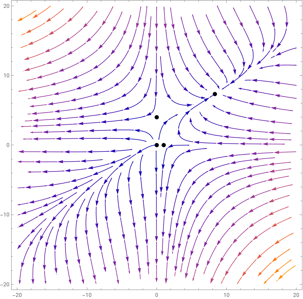
Given these parameters, the system generates the saddle path equilibrium in the vicinity of one of the four steady state values, whereas the remaining three become sources. This means that the balanced growth of the two variables is hard to attain unless and until a careful planning puts the growth of these two variables on a balanced path.
An interactive visualization of the growth of the physical capital stock, the stock of knowledge, and of production of final goods
An interactive visualization of the growth of the physical capital stock, the stock of knowledge, and of production of final goods
Introduction
Introduction
Up until now, we have focused on the core model structure and the derivation of a system of two nonlinear differential equations that describes the interaction between the change in the stock of knowledge and the growth of the capital stock.
In this section, we design and construct interactive models that show the dynamic solution curves of both the stock of knowledge, the capital stock, and the quantity of final goods produced. We continue to assume that the representative firm allocates two inputs -- both the capital stock and labor input -- to both the R&D sector and the final goods production sector. If the firm successfully invents a new stock of knowledge that is directly applicable to the final goods production sector, it will increase the productivity of both the capital and labor input in this sector, thereby producing a greater quantity of final goods. How exactly the invention and application of this new stock of knowledge in the final goods production sector will boost output in the latter sector depends on some crucial parameters explained below.
For the analytical purpose, this section considers first one simple case in which the representative firm recruits a group of talented workers for its R&D activity. This R&D activity is done by this special group of talented workers without a substantial investment or allocation of the physical capital stock. Therefore, the firm’s decision is about how much labor input to allocate to this R&D sector; in the subsequent sub-section, we introduces the possibility that the firm makes a decision about allocating both the capital stock and the labor input to both the R&D and the final goods production sector.
The allocation of labor input only
The allocation of labor input only
Suppose that the firm’s R&D sector does not utilize the fixed capital stock. A group of talented workers (i.e., scientists and engineers) brainstorm and conduct their R&D to invent a new production technology. In this case, the production function for the final goods production sector and the R&D sector will be, respectively:
A
γ
(sRL(t))
θ
(t)
α
=[A(t)(1-sR)L(t)]
(
12
)For computational ease, we replace the labor allocation parameter with sR, meaning share of labor in R&D sector. The following syntax enables us to create an interactive chart:
a
L
In[]:=
Clear[eqn1,sol1,A,Y,B,theta,gamma,alpha,sR,L,A0,Y0,Y,t];Manipulate[Module[{eqn1,sol1,A,Y},eqn1={A'[t]==B*(sR*L)^gamma*A[t]^theta,A[0]==A0};sol1=NDSolve[eqn1,A,{t,0,100}];Y[t_]:=(((1-sR)*L)*A[t]/.sol1[[1]])^alpha;GraphicsGrid[{{Plot[Evaluate[A[t]/.sol1],{t,0,100},PlotRange->All,PlotStyle->{Thickness[0.007],Blue},AxesLabel->{"Time","A(t)"},PlotLabel->Style["The growth of the stock of Knowledge",14,Bold],GridLines->Automatic,ImageSize->350],Plot[Evaluate[Y[t]],{t,0,100},PlotRange->All,PlotStyle->{Thickness[0.007],Red},AxesLabel->{"Time","Y(t)"},PlotLabel->Style["The growth of output",14,Bold],GridLines->Automatic,ImageSize->350]}},ImageSize->800]],Style["Allocation of Labor Input",Bold,14],{{sR,0.2,"Labor share to R&D (sR)"},0,0.9,0.01,Appearance->"Labeled"},{{L,100,"Total labor input (L)"},10,500,10,Appearance->"Labeled"},Delimiter,Style["The R&D Sector",Bold,14],{{A0,10,"Initial knowledge (A0)"},1,50,1,Appearance->"Labeled"},{{B,0.02,"Level effect of existing A (B)"},0.01,0.1,0.001,Appearance->"Labeled"},{{theta,0.6,"Spillover on new knowledge(θ)"},0.3,1.4,0.1,Appearance->"Labeled"},{{gamma,0.5,"Labor productivity in R&D (γ)"},0.1,0.9,0.1,Appearance->"Labeled"},Delimiter,Style["The Final Goods Production Sector",Bold,14],{{alpha,1.0,"Intensity of effective labor(α)"},0.5,1.5,0.1,Appearance->"Labeled"},TrackedSymbols:>True,SaveDefinitions->True]
The allocation of both the capital stock and labor input
The allocation of both the capital stock and labor input
Suppose now that the firm allocates its two input to both the R&D sector and the final goods production sector. The production function for the final goods production sector and the R&D sector will be, respectively:
With these modifications of the notation, we can use the following syntax for creating interactive charts:
Conclusion
Conclusion
In this notebook, we have sought to reconstruct Paul Romer’s new growth model. One crucial innovation is that the change in A is no longer an exogenous variable. Rather, the growth of the A-term is treated as a result of the representative firm’s deliberate efforts to invent a new stock of knowledge in the R&D sector. The development of a stock of new knowledge then positively affects the final goods production sector. We examined this idea by inferring the system of two nonlinear differential equations and by creating interactive charts that show how the interaction between the two sectors can alter the growth trajectory of the final goods producing sector.
One thing that is not obvious in this dynamic simulation exercise is that there is no particular mechanism for ensuring a balanced growth path between the R&D sector and the final consumption goods production sector. Instead, the phase diagram analysis implies that the model economy may or may not attain the steady state growth path. It is logically possible that the production of either final consumption goods or the stock of knowledge can be disproportional unless and until there is a coordinated effort to put them on a balance growth path.
Finally, this endogenous growth model also suffers from the same fundamental aporia that we identified in the previous session: It is about the very interpretation of the A-term. If we recall the fact that the A-term is nothing more than a weighted average of constant income distribution parameters, Romer’s endogenous growth model ends up presenting an idiosyncratic conclusion that firms are proactively allocating their scarce and costly resources to affect the internal distribution of corporate income.
Reference
Reference
◼
Paul M. Romer, “Increasing Returns and Long-Run Growth,” Journal of Political Economy, Vol. 94 (1986), pp.1002–1037.
◼
-------------------, “Endogenous Technical Change,” Journal of Political Economy, Vol. 98 (1990), pp.71-102.
◼
David Romer, Advanced Macroeconomics, McGraw-Hill, 2011 (4th edition), Ch. 3.
◼
Srinivas Raghavendra and Petri T. Piiroinen, An Introduction to Economic Dynamics - Modelling, Analysis and Simulation, Routledge: 2023, pp.143-159.
Appendix
Appendix
This appendix is designed to explore the possibility to introduce a stochastic variation term in the growth of A. As we saw in the previous session, the representative RBC theorists modified the Solow production function by introducing a stochastic term inside the A-term. Similar to that idea, we can introduce the same stochastic variation term in the evolution of the production of the stock of knowledge in Romer’s growth model setting. Simply put, we want to experiment with combining the RBC’s core ideas with Romer’s endogenous knowledge production.
Suppose the stochastic variation term follows the same Brownian Motion process with a drift = 0 and volatility = sigma. With this new term, the differential equation for A(t) and the production function for the final output are modified accordingly. As in the previous RBC models, Romer’s endogenous growth model is now affected by this volatility term appearing the production of the stock of knowledge. The production function in the final goods sector and the change in the stock of knowledge now become:
The following syntax can help us control this volatility parameter, sigma:
CITE THIS NOTEBOOK
CITE THIS NOTEBOOK
Introduction to dynamic economic models: Romer's endogenous growth model
by Hee-Young Shin
Wolfram Community, STAFF PICKS, January 13, 2026
https://community.wolfram.com/groups/-/m/t/3605935
by Hee-Young Shin
Wolfram Community, STAFF PICKS, January 13, 2026
https://community.wolfram.com/groups/-/m/t/3605935