Wolfram Cloud Document

ABSTRACT (original article): The Technology-Enhanced Learning (TEL) Marketplace was a joint initiative by the vice rectorate for academic affairs and the vice rectorate for digitization and change management at Graz University of Technology to modernize lectures. As part of this initiative, an exercise course on chemical thermodynamics was redesigned as a learner-centered course and enriched with interactive learning materials designed to promote self-directed learning. The core of the method used to implement this redesign is interactive notebooks created in Wolfram Mathematica to enable students to work through the examples independently, in depth, and irrespective of time, with the required theoretical background integrated into the notebooks. In this paper, we ask the following questions: RQ1: How did students use and accept the interactive notebooks? RQ2: What was the impact of the interactive notebooks and the corresponding course design as perceived by the students? To answer these questions, we conducted a questionnaire-based survey with 45 course students and statistically analyzed the results. Key results for RQ1 show that 93.33% of the participating students reported using the interactive notebooks, and technology acceptance (1 = low TA, 5 = high TA) was high in both the dimensions of perceived usefulness (𝑚 =3.88) and attitude (𝑚 =4.24). Regarding RQ2, our key results show that students perceived the notebooks to have a positive impact on their learning experience, especially regarding their self-directed learning. The results of this work are in alignment with observations by lecturers, which showed that this more student-centric course design and the integration of the interactive learning materials made it possible to clarify detailed questions during the independent learning phase, allowing the interactive part of the course to focus on the tactical approaches, solutions, and problems that arose during the calculations, which raised the overall level of content teaching. CITATION (original article): Haring, M.; Bangerl, M.M.; Wallek, T. Exploring the Impact of Self-Directed Learning with Interactive Notebooks on Students’ Experiences in a Chemical Thermodynamics Exercise. Educ. Sci. 2025, 15(10), 1334; https://doi.org/10.3390/educsci15101334

Interactive Book “Chemical Thermodynamics I” Abstract: This course aims at equipping the students with the theoretical basics and most relevant practical methods and models of chemical thermodynamics. Thus they are enabled to understand and to apply the various approaches which are commonly used for estimation of thermodynamic properties and phase equilibria. Furthermore, they are able to recognize both the possibilities and limits of different thermodynamic approaches that are used for layout of unit operations and plants. The lecture adopts, wherever possible, an integrated approach for developing chemical thermodynamics from both the classical and the statistical - mechanical viewpoint and to explain bulk phenomena of non - ideal systems as consequences of interactions on the molecular level.

This book acts as supplementary teaching material next to the lectures focusing on interactive plots to visualize otherwise unclear content .

Full book is available for download at the end of this post in CDF format. The ‘Wolfram Player’ is free of use and can open cdf files. It is available at https://www.wolfram.com/player/

Sample Chapter 2 of the book

Estimation of Critical Data with Joback

Shown by a dynamic calculation module

2023 02 07 Maintained by Thomas Wallek

Description

In chemical thermodynamics, it is often important to know (or estimate) the critical point of a component, since many models are based on this information. The estimation method by Joback is a so-called ‘group contribution’ method that estimates the critical data based on the number and kind of increments the molecule consists of. It is important to determine the correct increments a molecule consists of.

The manipulation module below can be operated by entering the number of increments your component has.
Simply click the “+“ and “-“ buttons to add or remove increments of a certain type.
The window to the left then shows the calculation for the estimation with Joback’s method for the critical data.

Background Information

◼

Formulae

T b = 198 + ∑ ΔT b	[K]	n A	...	number of atoms in the molecule
T f = 122 + ∑ ΔT f	[K]
T C = T b ·[0.584 + 0 ΔT C - ∑ ΔT C 2 ) -1 ]	[K]
P c = 0.113 + 0 n A - ∑ ΔP C -2 )	[bar]
v c = 17.5 + ∑ Δv c	[ 3 cm /mol]

◼

Tables for

ΔT

ΔP

and

Δv

Nonring increments

Ring increments

Halogen increments

Oxygen increments

Nitrogen increments

Sulfur increments

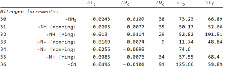
Manipulate

Index	Name	Number
Non Ring Increments:
1	- CH 3	- 0 +
2	> CH 2	- 0 +
3	>CH-	- 0 +
4	>C<	- 0 +
5	= CH 2	- 0 +
6	=CH-	- 0 +
7	=C<	- 0 +
8	=C=	- 0 +
9	≡CH	- 0 +
10	≡C-	- 0 +
Ring Increments:
11	- CH 2 -	- 0 +
12	>CH-	- 0 +
13	>C<	- 0 +
14	=CH-	- 0 +
15	=C<	- 0 +
Halogen Increments:
16	-F	- 0 +
17	-Cl	- 0 +
18	-Br	- 0 +
19	-I	- 0 +

Index	Name	Number
Oxygen Increments:
20	-OH (alcohol)	- 0 +
21	-OH (phenol)	- 0 +
22	-O- (nonring)	- 0 +
23	-O- (ring)	- 0 +
24	>C=O (nonring)	- 0 +
25	>C=O (ring)	- 0 +
26	O=CH- (aldehyde)	- 0 +
27	-COOH (acid)	- 0 +
28	-COO- (ester)	- 0 +
29	=O (except as above)	- 0 +
Nitrogen Increments:
30	- NH 2	- 0 +
31	>NH (nonring)	- 0 +
32	>NH (ring)	- 0 +
33	>N- (nonring)	- 0 +
34	-N= (nonring)	- 0 +
35	-N= (ring)	- 0 +
36	-CN	- 0 +
37	- NO 2	- 0 +
Sulfur Increments:
38	-SH	- 0 +
39	-S- (nonring)	- 0 +
40	-S- (ring)	- 0 +

∑Δ T B = 0	∑Δ T B = 0.
T B = 198 + ∑ ΔT B	T B = 198. K
∑Δ T F = 0	∑Δ T F = 0.
T F = 122 + ∑ ΔT F	T F = 122. K
∑Δ T C = 0	∑Δ T C = 0.
T C = -1 0.584 + 0.965·∑ ΔT C - 2 (∑ ΔT C ) 	T C = 339.041 K
∑Δ P C = 0	∑Δ P C = 0.
P C = -2 (0.113 + 0.0032· n A -∑ ΔP C )	P C = 78.3147 bar
∑Δ v C = 0	∑Δ v C = 0.
v C =17.5+∑ Δv C	v C = 17.5 3 cm /mol

Phase Diagram of Pure Fluids

Shown by a dynamic plot

2023 02 07 Maintained by Thomas Wallek

SetDirectory[ParentDirectory@NotebookDirectory[]];(*LoadPackagesfromsubfolder'pkg/'*)Needs["PropertyPackage`",FileNameJoin[{"pkg","PropertyPackage.wl"}]];Needs["ChemicalThermoPackage`",FileNameJoin[{"pkg","ChemicalThermoPackage.wl"}]];Unprotect["PropertyPackage`*"];

Description

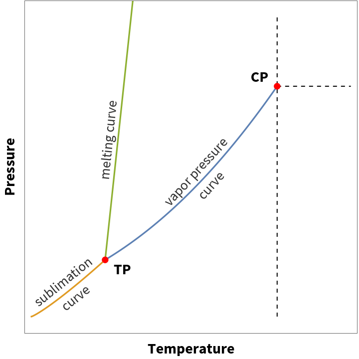
A phase diagram is a type of chart that shows the conditions (temperature, pressure, volume, composition, etc. ) at which a certain phase is most stable. We distinct phases of a pure component between solid, liquid, vapor, gas and supercritical fluid.
A simple example of a phase diagram is the PT-diagram (pressure over temperature).
The phase areas are divided by the sublimation, melting and condensation curve, called so after the individual phase change.
The condensation curve will more often be referred to as the ‘vapor pressure’ or ‘saturation pressure’ curve.
The triple point is where the sublimation, melting and vapor pressure curves meet. It is called ‘triple point’ because all 3 phases (solid, liquid, vapor) are present at the same time.
The critical point denotes the change to a supercritical fluid. The attributes of a supercritical fluid can differ from a regular gas or vapor.

At any given temperature one can also draw the phase diagram with changing molar volume to result in a Pv-diagram (pressure over molar volume). Here, the phase areas are divided by the saturated liquid and saturated vapor line in addition to the critical point.
The area between the saturated liquid and saturated vapor line is a two-phase area, which means that both vapor and liquid will be present. The isothermal line a the critical temperature denotes the border to the gas / supercritical fluid area.

The manipulation plot below displays an example PT- and PV-diagram for a pure component.
Move the locator object (“⊕”) with your mouse to different areas in the diagram.
The framed box above the diagram will display the most stable phase at the specified pressure and temperature/molar volume.

Manipulate

◼

Function Definition



ManipulatePlotPurePhaseDiagram[]

Axes of the Phase Diagram:

PT-Diagram

PV-Diagram

Stable Phase at Locator:

Vapor

Legend:CP ... critical pointTP ... triple point

Sensitivity of the Antoine Equation

Shown by means of an example

2023 02 07 Maintained by Thomas Wallek



Description

The Antoine equation is one of the most frequently used models for calculating the saturation pressure of components.
It depends on 3 parameters (A, B, C), making it relatively easy to fit to experimental data.
The Antoine parameters for methane are displayed below for reference.

Each of the 3 parameters of the Antoine equation influences the course of the saturation pressure curve differently.
Explore the sensitivity of the calculated saturation pressure with respect to varying parameter values in the manipulation plot below.
You will see that the first parameter A has a much higher influence on the resulting curve than any other parameter.

Background Information

Antoine parameters of Methane:

Methane
Antoine Parameter:
Units:	" log 10 ,K,bar
A =	3.9895
B =	443.028
C =	-0.49

Manipulate

CITE THIS NOTEBOOK

Self-directed learning with notebooks students' experiences in a chemical thermodynamics exercise
by Michael Haring, Mia Magdalena Bangerl & Thomas Wallek
Wolfram Community, STAFF PICKS, February 24, 2026
https://community.wolfram.com/groups/-/m/t/3644671