Dynamics of two tanks in seriesAuthors: Housam Binous and Ahmed Bellagi
Dynamics of two tanks in seriesAuthors: Housam Binous and Ahmed Bellagi
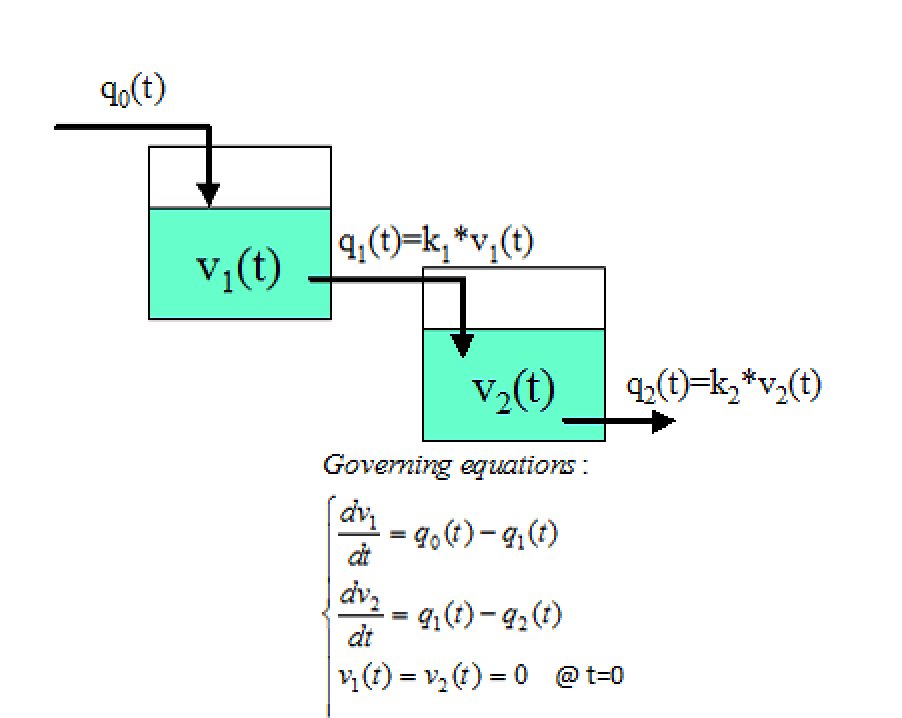
Assume volumetric flow rate proportional to liquid volume in the tank :
(t)=(t) where i=1, 2. Initially the two tanks are empty.
q
i
k
i
v
i
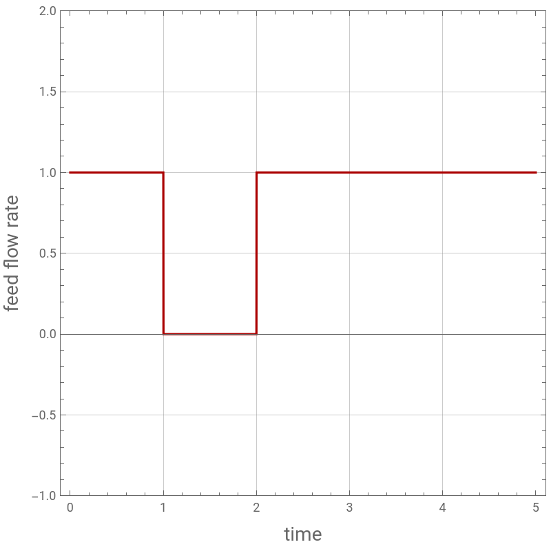
Feed flow rate is constant equal to 1 except between t = β and t = 2 β where it drops to zero.
In[]:=
q
0
In[]:=
Plot[[t]/.β1,{t,0,5},PlotStyleDarker@Red,AspectRatio1,GridLinesAutomatic,FrameTrue,ImageSize400{1,1},PlotRange{-1,2},FrameLabel{Style["time",14],Style["feed flow rate",14]}]
q
0
Out[]=
Numerical solution of the governing equations for β = 1 and =k=1.
k
i
In[]:=
sol=NDSolve[{(D[[t],{t,1}][t]-k[t])/.β1/.k1,(D[[t],{t,1}]k[t]-k[t])/.β1/.k1,[0]0,[0]0},{[t],[t]},{t,0,10}]
v
1
q
0
v
1
v
2
v
1
v
2
v
1
v
2
v
1
v
2
Out[]=
[t]InterpolatingFunction[t],[t]InterpolatingFunction[t]
v
1


v
2

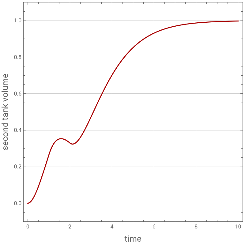
Plotting volume of the second tank versus time
In[]:=
plt1=Plot[[t]/.sol,{t,0,10},PlotStyleDarker@Red,AspectRatio1,GridLinesAutomatic,FrameTrue,ImageSize400{1,1},PlotRange{-0.1,1.1},FrameLabel{Style["time",14],Style["second tank volume",14]}]
v
2
Out[]=
An analytical solution for can be obtained using Laplace Transform.
v
2
Eliminating , one gets the following second order ODE:
v
1
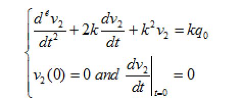
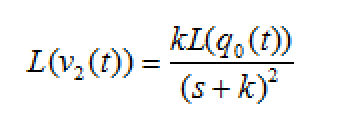
Taking the Laplace Transform, one gets :
In[]:=
Q[s]=LaplaceTransform[[t]/.β1,t,s]
q
0
Out[]=
1
s
-2s
s
-s
s
Taking the Inverse Laplace Transform, one obtains an expression for the volume of the second tank.
In[]:=
IV=InverseLaplaceTransform[k/(s+k)^2Q[s],s,t]
Out[]=
1
k
-k(-2+t)
k(-2+t)
-kt
kt
kt
k
In[]:=
laplac
2
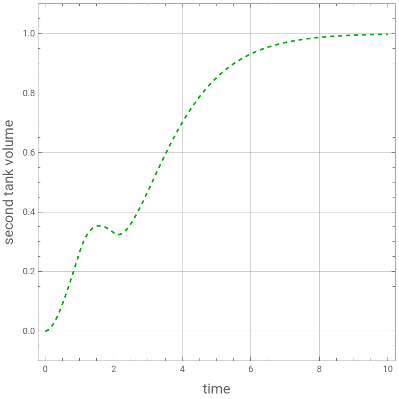
Plotting the analytical solution for (t).
v
2
In[]:=
plt2=Plot[[t]/.k1,{t,0,10},PlotStyle{Dashed,Darker@Green},PlotStyleDarker@Red,AspectRatio1,GridLinesAutomatic,FrameTrue,ImageSize400{1,1},PlotRange{-0.1,1.1},FrameLabel{Style["time",14],Style["second tank volume",14]}]
laplac
2
Out[]=
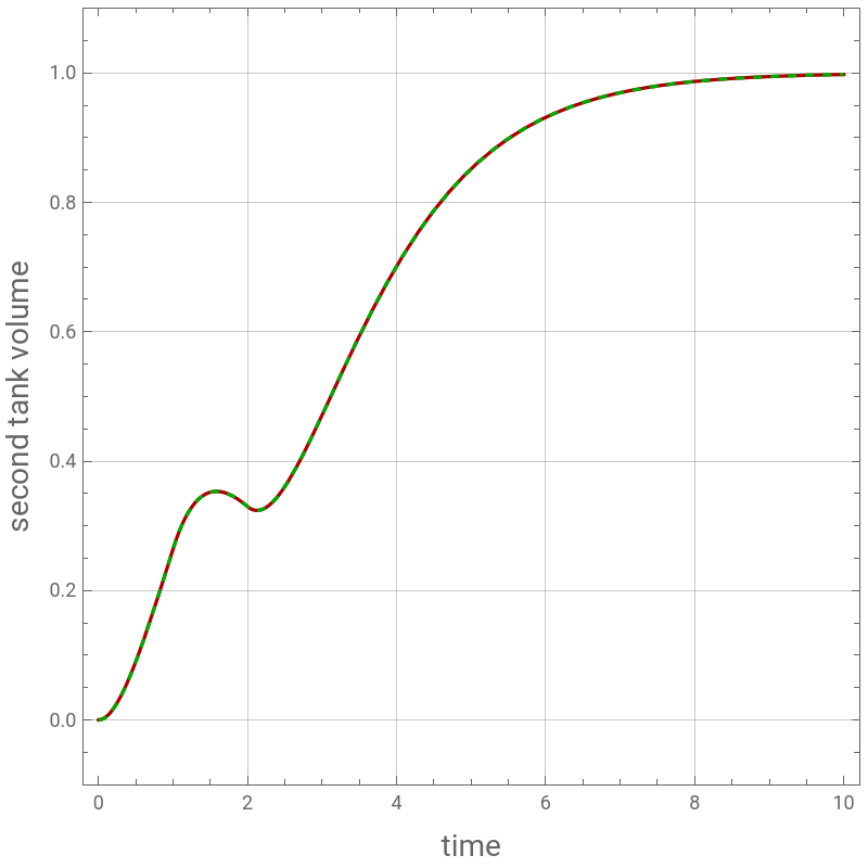
Comparing the numerical and analytical solutions
In[]:=
Show[plt1,plt2]
Out[]=