Based on J. Crank, The Mathematics of Diffusion, 2nd ed., Clarendon Press, Oxford, 1975, Section 5.3.3 (eqs. 5.33-5.35, Table 5.1, Fig. 5.7)
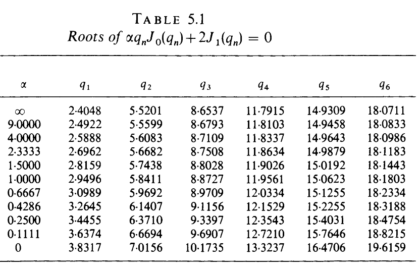
Physical problem (Crank, §5.3.3):A cylinder of radius a (occupying r < a) is immersed in a well-stirred bath of limited volume, whose cross-section is A (excluding the cylinder). The solute concentration in the bath is always uniform and equals C0 initially; the cylinder is initially free of solute. The total amount of solute taken up by the cylinder after time t, as a fraction of the amount after infinite time, is (Wilson 1948)and α = A/(π a^2) is the ratio of the volumes of solution and cylinder (α = A/(π a^2 K) if a partition coefficient K applies). α is tied to the final fractional uptake of solute by the cylinder throughCrank tabulates the first roots for several values of α (Table 5.1) to help evaluate (5.33), and Fig. 5.7 shows / against for final uptakes of 0, 30, 50, 70 and 90 percent. The series converges slowly for small , for which Crank gives alternative small-time expressions (5.36)-(5.41). The concentration inside the cylinder is given by (5.42), and the same equations describe desorption into a well-stirred solution when (5.35) is replaced by (5.43).
M
t
M
∞


q
n
M
t
M
∞
Dt/
2
a
Dt/
2
a
This notebook computes the roots of (5.34) as a function of a single parameter , where is the fraction of solute left in the bath at equilibrium ( means α = 0, i.e. 100% uptake; means α = Infinity, i.e. no uptake). Dividing (5.34) by (1 + α) gives the equivalent form used in the first cell (eq1):
m q J0(q) + 2 (1 - m) J1(q) = 0
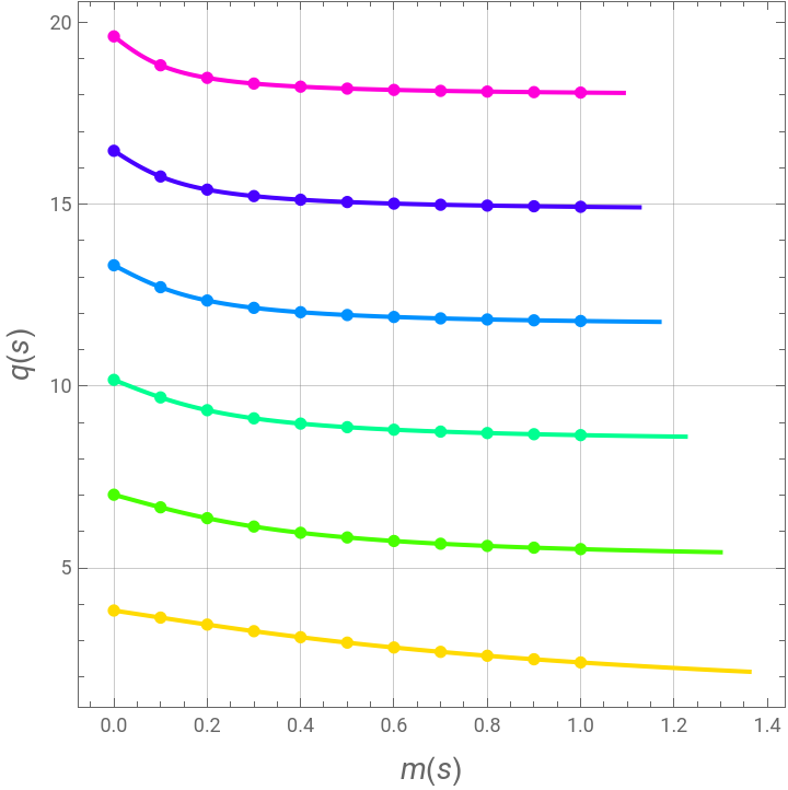
Each root branch(m) is a curve in the (m, q) plane. Rather than solving for at each separately, the notebook traces the whole curve parametrically: eq2 imposes arc-length parametrisation, m'(s)^2 + q'(s)^2 = 1, and NDSolve (function sol[k]) integrates the pair {m[s], q[s]} from the starting point m = 0, q = BesselJZero[1, k] (where J1(q) = 0, the α = 0 limit), for k = 1, 2, 3, ... This avoids the difficulty of root finding near turning points and gives all branches q_1, q_2, ... as smooth interpolating functions.
The list mus = {1, 9/10, ..., 1/10, 0} contains the values of m corresponding to the final uptakes 0%, 10%, ..., 100%. These are converted to the α values via α = m/(1 - m) (the first one being Infinity), and the interpolating solutions are then evaluated at each m to produce a table of α against q_1 ... q_6, in the same format as Crank's Table 5.1. The roots can then be used directly in the series (5.33) and (5.42) to reproduce the uptake curves of Fig. 5.7.
q
n
m
m=α/(1+α)=1-/(AC0)
M
∞
m=0
m=1
m q J0(q) + 2 (1 - m) J1(q) = 0
Each root branch
q
n
q
m
The list mus = {1, 9/10, ..., 1/10, 0} contains the values of m corresponding to the final uptakes 0%, 10%, ..., 100%. These are converted to the α values via α = m/(1 - m) (the first one being Infinity), and the interpolating solutions are then evaluated at each m to produce a table of α against q_1 ... q_6, in the same format as Crank's Table 5.1. The roots can then be used directly in the series (5.33) and (5.42) to reproduce the uptake curves of Fig. 5.7.
In[]:=
eq1=mqBesselJ[0,q]+2(1-m)BesselJ[1,q]==0/.m->m[s]/.q->q[s]
Out[]=
2BesselJ[1,q[s]](1-m[s])+BesselJ[0,q[s]]m[s]q[s]0
In[]:=
eq2=m'[s]^2+q'[s]^2==1
Out[]=
2
′
m
2
′
q
In[]:=
sol[k_]:=Quiet@NDSolve[{eq1,eq2,m[0]==0.0,q[0]==BesselJZero[1,k],q'[0]==0.1,m'[0]==0.1},{m,q},{s,-10,10},AccuracyGoal->5]
In[]:=
mus={1,9/10,4/5,7/10,3/5,1/2,2/5,3/10,1/5,1/10,0}
Out[]=
1,,,,,,,,,,0
9
10
4
5
7
10
3
5
1
2
2
5
3
10
1
5
1
10
In[]:=
alpha=N[Join[{Infinity},Drop[-mus,1.]/(Drop[mus,1]-1)],{5,4}]
Out[]=
{∞,9.000,4.000,2.333,1.500,1.000,0.667,0.429,0.250,0.111,0.×}
-4
10
In[]:=
tbl[k_]:=Flatten[Quiet@Table[FindRoot[(m[s]/.sol[k])==mus[[i]],{s,-1,0}],{i,1,Length@mus}],2]
In[]:=
tblf=Table[tbl[k],{k,1,6}]
Out[]=
{{s-1.75652,s-1.62371,s-1.48463,s-1.3379,s-1.18191,s-1.01491,s-0.835197,s-0.641693,s-0.434937,s-0.218502,s0.},{s-1.88804,s-1.78039,s-1.66926,s-1.55265,s-1.42724,s-1.28758,s-1.12493,s-0.926278,s-0.67516,s-0.360382,s0.},{s-1.9711,s-1.86788,s-1.76299,s-1.65527,s-1.54252,s-1.42039,s-1.28007,s-1.10387,s-0.858255,s-0.493076,s0.},{s-2.02935,s-1.92759,s-1.82489,s-1.72054,s-1.61311,s-1.49957,s-1.37299,s-1.21681,s-0.991447,s-0.610992,s0.},{s-2.07298,s-1.97188,s-1.87018,s-1.7674,s-1.6626,s-1.55362,s-1.43519,s-1.29336,s-1.08891,s-0.713234,s0.},{s-2.10728,s-2.00653,s-1.90536,s-1.80345,s-1.70012,s-1.59378,s-1.48041,s-1.3485,s-1.16192,s-0.800819,s0.}}
In[]:=
tbl2=Transpose@Join[{alpha},Table[First[q[s]/.Quiet@sol[j]/.(tblf[[j]][[i]])],{j,1,6},{i,1,11}]]
Out[]=
{{∞,2.40483,5.52008,8.65373,11.7915,14.9309,18.0711},{9.000,2.4922,5.55988,8.67929,11.8103,14.9458,18.0833},{4.000,2.58883,5.60829,8.71087,11.8337,14.9643,18.0987},{2.333,2.69618,5.66821,8.75082,11.8634,14.9879,18.1183},{1.500,2.81587,5.74378,8.80278,11.9026,15.0192,18.1443},{1.000,2.9496,5.84112,8.87272,11.9561,15.0624,18.1803},{0.667,3.0989,5.96923,8.9709,12.0334,15.1255,18.2334},{0.429,3.26454,6.14073,9.11565,12.1529,15.2255,18.3188},{0.250,3.44549,6.37095,9.33965,12.3543,15.4031,18.4754},{0.111,3.63743,6.66936,9.69067,12.721,15.7646,18.8215},{0.×,3.83171,7.01559,10.1735,13.3237,16.4706,19.6159}}
-4
10
In[]:=
TableForm[tbl2,TableHeadings->{None,{Style["α",Darker@Green,14],Style["q1",Darker@Red,14],Style["q2",Darker@Red,14],Style["q3",Darker@Red,14],Style["q4",Darker@Red,14],Style["q5",Darker@Red,14],Style["q6",Darker@Red]}},TableSpacing->{3,3}]
Out[]//TableForm=
α | q1 | q2 | q3 | q4 | q5 | q6 |
∞ | 2.40483 | 5.52008 | 8.65373 | 11.7915 | 14.9309 | 18.0711 |
9.000 | 2.4922 | 5.55988 | 8.67929 | 11.8103 | 14.9458 | 18.0833 |
4.000 | 2.58883 | 5.60829 | 8.71087 | 11.8337 | 14.9643 | 18.0987 |
2.333 | 2.69618 | 5.66821 | 8.75082 | 11.8634 | 14.9879 | 18.1183 |
1.500 | 2.81587 | 5.74378 | 8.80278 | 11.9026 | 15.0192 | 18.1443 |
1.000 | 2.9496 | 5.84112 | 8.87272 | 11.9561 | 15.0624 | 18.1803 |
0.667 | 3.0989 | 5.96923 | 8.9709 | 12.0334 | 15.1255 | 18.2334 |
0.429 | 3.26454 | 6.14073 | 9.11565 | 12.1529 | 15.2255 | 18.3188 |
0.250 | 3.44549 | 6.37095 | 9.33965 | 12.3543 | 15.4031 | 18.4754 |
0.111 | 3.63743 | 6.66936 | 9.69067 | 12.721 | 15.7646 | 18.8215 |
0.× -4 10 | 3.83171 | 7.01559 | 10.1735 | 13.3237 | 16.4706 | 19.6159 |
In[]:=
Show[Table[ParametricPlot[Evaluate[{m[s],q[s]}/.sol[j]],{s,-2.2,0},AspectRatio->1,Frame->True,GridLines->Automatic,PlotStyle->Hue[j/7]],{j,1,6}],Table[ListPlot[Table[First[{m[s],q[s]}/.Quiet@sol[j]/.(tblf[[j]][[i]])],{i,1,11}],PlotStyle->{Hue[j/7],PointSize[0.0175]}],{j,1,6}],PlotRange->All,FrameLabel->{Style[m[s],14],Style[q[s],14]}]
Out[]=