Playing with prime numbers and the Sine Function
In the first step of this process, the function getSum is defined. The objective of this function is to compute the sum of the sines, there will be terms, each of these will have either the integer prime number or the square root of it
i
In[]:=
getSum[i_Integer,t_]:=Module[{q},q=Table[Prime[r],{r,i}];Sum[Sin[t*x],{j,q}]]
First scenario Integer prime numbers in the argument
First scenario Integer prime numbers in the argument
Just prime numbers
Just prime numbers
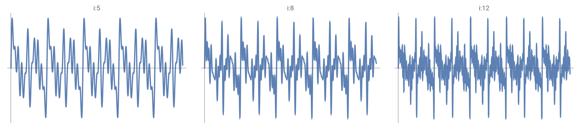
The following visualizes the sine wave behavior of the first 5, 8, and 12 prime numbers, which also corresponds to the number of terms in the sum, ranging from 0 to 30.
In[]:=
GraphicsRow[Table[Plot[getSum[i,j],{x,0,30},PlotTheme->"Minimal",PlotLabel->"i:"<>ToString[i]],{i,{5,8,12}}],ImageSize->Full]
Out[]=
Full range
Full range
Let’s compare with the case where goes from 1 to 5, 8, 12. This is, here we are showing the behavior of the function with the same number of terms, and not the range, for example, from 1 to the 5th prime number, that is a different case
i
In[]:=
GraphicsRow[Table[Plot[Sum[Sin[i*x],{i,j}],{x,0,30},PlotRange->Full,PlotTheme->"Minimal",PlotLabel->"i:"<>ToString[j]],{j,{5,8,12}}],ImageSize->Full]
Out[]=
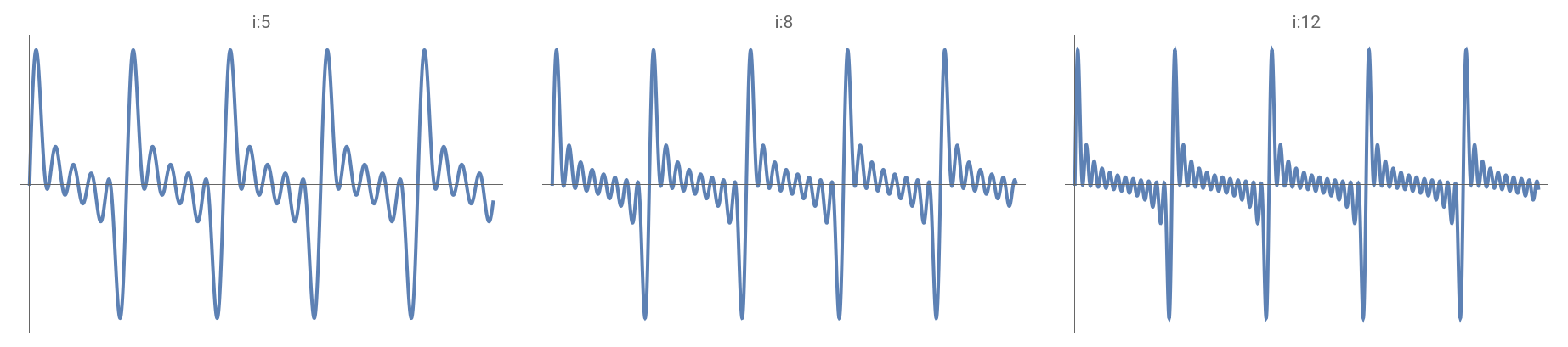
It has been noticed that when is limited to prime numbers, the resulting behavior is more erratic. The presence of more spikes, a greater variety of sizes, and a more challenging range to limit the behavior is also evident. It is evident that as the number of terms increases, the behavior remains significantly different. In the case where i is a number from 0 to j, the behavior approaches the x-axis. However, for prime numbers, the behavior does not converge to the x-axis.
i
Second scenario Square root of prime numbers in the argument
Second scenario Square root of prime numbers in the argument
Just primes
Just primes
The following visualizes the sine wave behavior where we have taken the square root of the first 5, 8, and 12 prime numbers, which also corresponds to the number of terms in the sum, ranging from 0 to 30.
In[]:=
GraphicsRow[Table[Plot[getSum[i,Sqrt[j]],{x,0,30},PlotTheme->"Minimal",PlotLabel->"i:"<>ToString[i],PlotRange->All],{i,{5,8,12,18}}],ImageSize->Full]
Out[]=

Full range
Full range
Let’s compare with the case where goes from 1 to 5, 8, and 12. Here again we are showing the behavior of the wave with the same number of terms
i
In[]:=
GraphicsRow[Table[Plot[Sum[Sin[Sqrt[i]*x],{i,j}],{x,0,30},PlotRange->Full,PlotTheme->"Minimal",PlotLabel->"i:"<>ToString[j]],{j,{5,8,12,18}}],ImageSize->Full]
Out[]=

As was the case previously, even in the context of random behavior, it is evident that prime numbers exhibit a heightened degree of randomness, manifesting as increased spikes and waves. To illustrate this phenomenon, consider the case of , where ranges from 1 to 18. Initially, the behavior is characterized by a smooth progression. However, in the case of a prime , the behavior undergoes a significant transformation, revealing more intricate structures.
i18
i
i
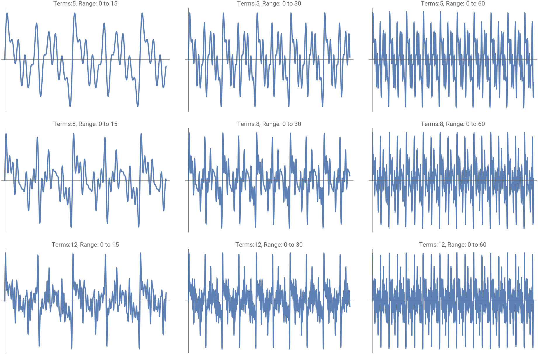
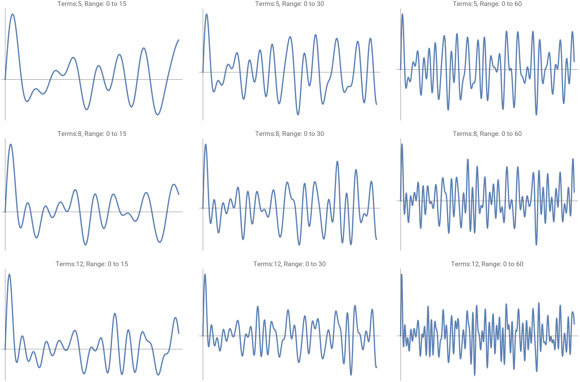
Third scenario Comparing different domains
Third scenario Comparing different domains
Prime integer parameter
Prime integer parameter
In[]:=
GraphicsGrid[Table[Plot[getSum[i,j],{x,0,k},PlotTheme->"Minimal",PlotLabel->"Terms:"<>ToString[i]<>", Range: 0 to "<>ToString[k],PlotRange->All],{i,{5,8,12}},{k,{15,30,60}}],ImageSize->Full]
Out[]=
Square root of primes
Square root of primes
In[]:=
GraphicsGrid[Table[Plot[getSum[i,Sqrt[j]],{x,0,k},PlotTheme->"Minimal",PlotLabel->"Terms:"<>ToString[i]<>", Range: 0 to "<>ToString[k],PlotRange->All],{i,{5,8,12}},{k,{15,30,60}}],ImageSize->Full]
Out[]=
Decimal Analysis
Here we analyze the decimal behavior to have a better understanding of what is happening, not just a visual representation, but also a numerical one. Here we are working just with prime numbers
First step Function getRange that returns the first p prime numbers
First step Function getRange that returns the first prime numbers
p
In[]:=
getRange[p_Integer]:=Table[Prime[k],{k,p}]
Second step Table of the decimal numbers
Second step Table of the decimal numbers
The following is the method for reading the rows: The first element is the number, the second element is the square root, the third element is the sine function with an integer parameter, and the fourth element is the sine function with a real parameter. It is noteworthy that the sequence of hyphens is followed by a repetition of this pattern.
The first two rows are constant, as they represent the number and its square root, respectively. Let’s check the third and fourth row for each case. The third row is always the same too, indeed, this is the case where the argument is an integer number, so the behavior is a repetitive wave, always has the same value in the same point, there is no variation on its value. The fourth row is dynamic, even at a constant point, due to the argument being the square root. This results in random behavior.
At this point, two methods of visualizing the behavior are available, in addition to a numerical method.
Let’s add a third way: Decimal behavior
Binary representation of the decimal numbers
In this section we expand our scope and work with the full range of numbers, not merely the prime numbers, thereby facilitating a comprehensive visualization of the behavior in question without the omission of any relevant details.
Here we plot the binary representation of the decimal numbers of the sine function, integer, and real numbers. The initial 100 values of the sine function over the span of the first three periods have been plotted.
Integer numbers
Integer numbers
The behavior in question is consistent and uniform, and that the visual representation remains constant.
Real numbers
Real numbers
This behavior is distinct, despite the fact that it is occurring at the same point. A discernible discrepancy in the patterns at the upper and lower regions of the black mountains is evident upon observation. This observation lends further credence to the hypothesis that the behavior manifests in a distinct manner in each instance.
Conclusion
It has been demonstrated that when the parameter is an integer, the behavior is repetitive. However, when the parameter is a real number, the behavior is not repetitive. In this post, the analysis is repeated with a specific kind of numbers: prime numbers. Based on the initial exploration with the sine function, it can be noticed that the behavior is more erratic, with spikes and more elaborate patterns appearing. It is noteworthy that the range of prime numbers is smaller than the natural numbers in the given range. However, the presence of fewer prime numbers in the range does not guarantee a simpler pattern. This finding is counterintuitive, as one might expect more complexity with a larger number of terms. However, this is not the observed pattern.
The decimal analysis revealed that the sine wave with integer values remain constant over each period. In contrast, parameters with real values exhibit variability, resulting in a different value for each period.
The final analysis confirmed the hypothesis that decimal numbers are not repetitive. Each case is unique, and this phenomenon could be applicable to specific fields, such as cryptography.