Cellular automaton vary in their behavior based on the given initial conditions and the defined rule. To further understand different patterns, I started with finding the rule for automatons by looking at the middle column generated from an initial singular black cell. I then explored the limits of unique middle columns that can be generated given various initial conditions. To more effectively account for the variety of patterns, I developed rule plots dynamically from a given automaton and then attempted to reverse the pattern to find the first row.
Understanding Cellular Automata
Understanding Cellular Automata
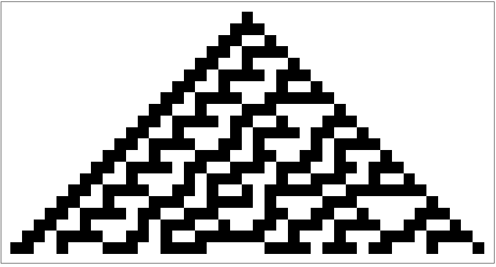
To start exploring the patterns that cellular automata creates, I used the ArrayPlot function to visualize rule 30.
Example with rule 30, starting with a singular black cell in a row of white, ran for 20 generations:
In[]:=
ArrayPlot[CellularAutomaton[30,{{1},0},20]]
In[]:=
For the purposes of having an example automaton to test later code with, I stored a sequence in plot.
Rule 30, starting with the same starting conditions of one black cell, ran for 100 generations:
In[]:=
plot=CellularAutomaton[30,{{1},0},100];
Visualizing the Middle Column for Cellular Automata
To further explore the characteristics of different 2d cellular automata rules, I compared the middle columns of sequences generated. All of the 256 rules for automaton were generated using a starting pattern of one black cell, and then were grouped by the unique middle column patterns found.
Defining a function that takes a cellular automaton and returns an ArrayPlot of the middle column:
In[]:=
findMiddleColumn[explot_]:=ArrayPlot[Transpose@{explot[[All,Ceiling[Length[explot[[1]]]/2]]]}]
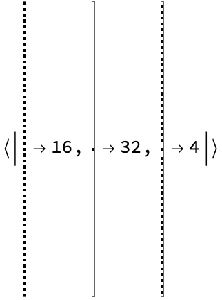
Using the Counts function and the above written findMiddleColumn function to loop through all 2d automaton rules to visualize the unique patterns (only 3 of the patterns are visualized below):
In[]:=
Counts[findMiddleColumn[CellularAutomaton[#,{{1},0},100]]&/@Range[255]][[1;;3]]
In[]:=
Rule from Middle Columns
Rule from Middle Columns
Instead of visually comparing all of the middle columns, I found the middle columns of all the rules in list form. Then, I developed an association with the rule number and the middle column pattern that it leads to with the initial condition of one black cell.
Defining a function that finds the middle column cell list without visualizing it in an array plot:
In[]:=
findMiddleColumnList[explot1_]:=explot1[[All,Ceiling[Length[explot1[[1]]]/2]]]
Mapping the function onto all the automaton patterns generated by 2d rules that start with one black cell:
In[]:=
allMiddleColumns=findMiddleColumnList[CellularAutomaton[#,{{1},0},100]]&/@Range[255];
Threading the association to see which rule corresponds to which pattern:
In[]:=
associationOfPatterns=AssociationThread[{#}&/@Range[255]->allMiddleColumns];
Once the information about the middle column patterns was collected for all the rules, I began comparing the middle columns of any given automaton (in this case, using the example of rule 30 with 100 generations and one black starting cell) with the association to find the nearest match to the rule being used to generate the given automaton.
Finding the Nearest Rule
Finding the Nearest Rule
Defining a function that checks for the nearest middle column to the middle column of the automaton given:
In[]:=
compareMiddleColumns[automaton_]:=Nearest[allMiddleColumns,findMiddleColumnList[automaton]];
In[]:=
Grid[Transpose[compareMiddleColumns[plot][[All,1;;10]]]]
In[]:=

Determining which rules correspond to the nearest middle columns found by finding the keys for the values in the association:
In[]:=
rules=Flatten[PositionIndex[associationOfPatterns][compareMiddleColumns[plot][[1]]]]
Out[]=
{30,86}
Visualizing Automata Results
Visualizing Automata Results
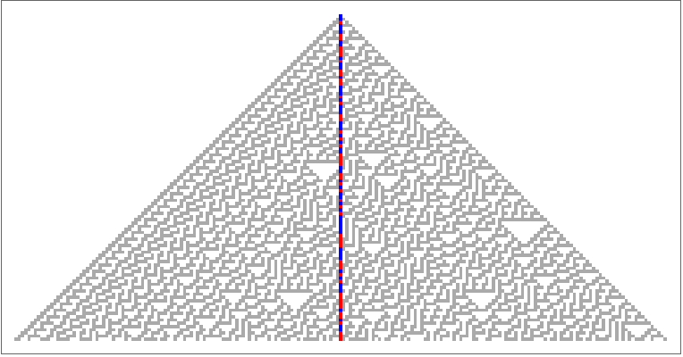
Once the nearest rules were found, I visualized the results of a sequence generated using the found rule and the original automaton given. I highlighted the center column of each using different color rules in order to express the match.
Defining a function that replaces the center column with different values so that different color rules can be applied:
In[]:=
centerReplacer[rule_Integer]:=Module[{center},center=Ceiling[Length[CellularAutomaton[rule,{{1},0},100][[1]]]/2];ReplacePart[#,If[#[[center]]==0,2,3],center]&/@CellularAutomaton[rule,{{1},0},100]]
Defining a function that finds the best rule and creates a visualization by replacing the center column of the image with changed color values:
In[]:=
visCompareMiddleColumns[automaton1_]:=(currMiddleColumn=findMiddleColumnList[automaton1];bestFind=Nearest[allMiddleColumns,currMiddleColumn];ruleNumber=PositionIndex[associationOfPatterns][bestFind[[1]]][[1]];ArrayPlot[centerReplacer[ruleNumber[[1]]],ColorRules->{2->Red,3->Blue}])
Generating the image:
In[]:=
picture=visCompareMiddleColumns[plot]
In[]:=
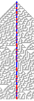
Cropping the image for better focus:
In[]:=
croppedPicture=ImagePad[picture,{{-300,-300},{-10,-10}}]
In[]:=
Visualizing the found matched columns alone side-by-side:
In[]:=
ImageCollage[Table[findMiddleColumn[CellularAutomaton[rules[[n]],{{1},0},15]],{n,1,2}]]
In[]:=

Putting all the visualizations together, including the center column alone, the highlighted column in the generated automaton, and the original automaton:
Unique Sequences with Varying Initial Conditions
Unique Sequences with Varying Initial Conditions
Though exploring the center columns of 2d automaton patterns with the same starting conditions was effective in being able to find a rule match for a given pattern, this changes as the initial conditions begin to differ. To study this, I looked at multiple different starting conditions by increasing the number of black cells in the starting row, and saw how many unique middle column patterns would be generated.
Adding more starting conditions (having one black cell, two black cells, and three black cells for all the rules now) and seeing the unique middle columns that can be generated:
Through this, I was able to see that the middle column patterns do begin to repeat and there is an asymptote that will be reached for the number of unique sequences that can possibly be generated.
Counting the number of unique center columns found when iterating through the initial starting conditions of 1 black cell, 2 black cells, and 3 black cells:
Defining a function that gets the total unique patterns for center columns based on different initial conditions for 10 generations (increasing the number of black cells to start with):
Finding the Maximum Unique Patterns
Finding the Maximum Unique Patterns
To visualize the point at which additional unique center column patterns stop being generated, I found the total types formed with 30 different initial conditions and then graphed the results.
Generate a list of the number of unique middle columns based on the number of starting black cells and store as the y-values:
Generate a list of the number of black starting cells as the x-values:
Develop this into a graph that depicts the relationship between the total unique combinations generated as the number of initial black cells increases:
For all of the 2d cellular automaton rules ran at 10 generations, the maximum number of unique sequences generated by increasing the initial number of black starting cells was 434, which is the found asymptote for these conditions.
Finding Rules from Unknown Cellular Automata
Finding Rules from Unknown Cellular Automata
Instead of comparing center column sequences to find matching rules, a more accurate way is to generate a rule plot dynamically. This allows for any random initial condition to be analyzed. With the rule plot, I then planned to figure out the initial row being given the rest of an automaton pattern.
Generating a random sequence for testing the code:
Cropping out the first row so that I can test finding it using my developed rule plot later:
Getting the list form of the above automaton pattern:
Generating the index combinations of the 3 cells that control each cell in the next row:
Grouping the indexes of the cells that control each of the cells in the next row:
To see what the different combinations of 3 cells lead to, I found all the possible unique combinations in the given automaton and then found what cell values they result in.
Getting all the groupings of 3 cells:
Initializing an empty rule plot association:
Adding all the unique rules into the rule plot (there are a total of 8 combinations and what cell values they lead to):
Successfully generated rule plot:
Determining the Initial Conditions
Determining the Initial Conditions
Since I had the rule plot generated from the automaton pattern, I began trying to apply the rules in reverse to find the initial row conditions. I started by determining which rules could lead to each cell in the second row.
Look at all of the cells in the second row and see what combinations can lead to that cell state:
Generate an empty table of combinations that the initial conditions could be:
Based on the options list, I then determined all of the possible patterns that the first row could be based on how each cell in the following row can be generated.
Loop through all of the possible combinations and then format them to show how all of the possible patterns look:
The next step is to check if any of the columns have the same element, since that would mean that the value of that cell has to be the correct value for that position in the initial row.
Transpose generationCombinations, and put the lists in matrix form so they are easier to visualize:
The transposed matrices are now easy to traverse to find fully repeated rows.
Check for any rows in the matrices that have all of the same elements by looping through (besides blank spaces):
From this list of boolean values, find the position of all the True values so that the fully repeated rows can be identified.
Check to see if any of the returned values are true, which would indicate that a cell at a certain index was confirmed with its value:
No fully repeated columns were found for any of the possible solutions, so I started to approach finding the right pattern by seeing which one satisfies all of the cell's conditions.
Defining a list of matrices that each contain the possible patterns based on each cell in the row:
In order to successfully visualize the combinations found, I assigned new color values to the unknown cells.
Replace the blank (underscore) values with the integer 2, so the color rule can be changed:
Putting all of the matrix values in ArrayPlots for visualization:
My next approach was to find the possible links between the combinations across the matrices. To do this, I subtracted each matrix with its adjacent matrix (matrix 1 and matrix 2 were subtracted, matrix 2 and matrix 3 were subtracted, etc.). I replaced the blank spaces with an arbitrary integer, in this case 9, so that the matching patterns would be the ones that do not have 1 or negative 1, since that would mean that a 0 and a 1 were subtracted and the patterns don't match in those positions.
Replace the blank (underscore) values in generationCombinations to the arbitrarily chosen integer 9:
Loop through all of the matrices that need to be subtracted and store the results:
Next, I checked through which of the subtractions in resulted in all values of the row not being 1 or -1.
Initializing an empty table with True to test which subtractions show that the patterns match:
Looping through the resultsOfSubtract to see which patterns fail to show a match, and changing their respective value to False in finding:
Once the successful subtractions were found, I worked backwards to see which indexes in the generationCombinations led to the True results in finding.
Initializing an empty list to store the indexes:
Looping through finding to see which indexes are being referred to:
I then used the indexes found to see what is being referred to in generationCombinations, and I put the subtracted pairs together so that they could be "linked". This results in an organized list of initial row combinations that work successfully with each other.
Initializing an empty list to store the pairs:
Looping through all of the indexesThatWork, seeing what they reference in generationCombinations, and appending the pairs to workingPatterns:
I took the workingPatterns list and developed a visualization for it in order to highlight the matches found.
Creating an association with the pairs of workingPatterns and using ArrayPlot to highlight the unknown missing values:
Future Plans
Future Plans
In conclusion, I was able to successfully use middle columns patterns from varying automaton to identify rules and was able to dynamically generate rule plots from any given automaton. I was also able to study the limits of unique middle column patterns that can be generated given various initial conditions.
Since I was not able to finish finding the right initial conditions, I would like to expand on that. The method that I plan on using is to take the pairs and find the longest chain of patterns, which could then be checked with the rule plot and confirmed to be the correct initial condition. Upon some cursory research, I have seen that the most effective way to accomplish this is to create a graph with the connections and find the longest path.
Since I was not able to finish finding the right initial conditions, I would like to expand on that. The method that I plan on using is to take the pairs and find the longest chain of patterns, which could then be checked with the rule plot and confirmed to be the correct initial condition. Upon some cursory research, I have seen that the most effective way to accomplish this is to create a graph with the connections and find the longest path.
Acknowledgements
Acknowledgements
I would like to thank my mentor Simeon for helping me throughout my project and everyone at the program for the support.
CITE THIS NOTEBOOK
CITE THIS NOTEBOOK
Find the simplest cellular automaton to generate a given sequence
by Twisha Patel
Wolfram Community, STAFF PICKS, July 13, 2023
https://community.wolfram.com/groups/-/m/t/2963085
by Twisha Patel
Wolfram Community, STAFF PICKS, July 13, 2023
https://community.wolfram.com/groups/-/m/t/2963085