For an overview of the finite element method functionality provided by the Wolfram language also see
https://www.wolfram.com/language/core-areas/finite-element-method/
https://www.wolfram.com/language/core-areas/finite-element-method/
NDSolve
NDSolve
◼
Ordinary Differential Equations
◼
Boundary Value Problems
◼
Delay Differential Equations
◼
Hybrid and Discontinuous Equations
◼
Differential-Algebraic Equations
◼
Partial Differential Equations
◼
Rectangular Regions
◼
Arbitrary Regions
Why Finite Elements
Why Finite Elements
Arbitrary shaped domains
Arbitrary shaped domains
Large class of PDEs
Large class of PDEs
Solving PDEs
Solving PDEs
Problem setup
Problem setup
◼
{x,y,..}∈Ω
◼
PDE
◼
Γ
NDSolve
NDSolve
Specification
Specification
- 2 ∇ |
Ω∈Disk |
Γ D |
Setup
Setup
In[]:=
pde=-u[x,y]==1;
2
∇
{x,y}
In[]:=
Ω=Disk[];
In[]:=
Γ
D
Solve
Solve
In[]:=
uif=NDSolveValue[{pde,},u,{x,y}∈Ω]
Γ
D
Out[]=
InterpolatingFunction


Visualize
Visualize
In[]:=
Plot3D[uif[x,y],{x,y}∈Ω]
Out[]=

Specific PDEs
Specific PDEs
CoefficientForm:mu+du+∇·(-c∇u-αu+γ)+β·∇u+au=f
2
∂
∂
2
t
∂
∂t
Laplace:∇·(-c∇u-αu+γ)+β·∇u+au=0
Poisson:∇·(-c∇u-αu+γ)+β·∇u+au=f
Helmholtz:∇·(-c∇u-αu+γ)+β·∇u+au=f
ConvectionDiffusionReaction: ∇·(-c∇u-αu+γ)+β·∇u+au=f
Heat:u+u+∇·(-c∇u-αu+γ)+β·∇u+au=f
2
∂
∂
2
t
∂
∂t
Wave:u+u+∇·(-c∇u-αu+γ)+β·∇u+au=0
2
∂
∂
2
t
∂
∂t
Poisson’s equation
Poisson’s equation
PDE
Poisson:∇·(-c∇u-αu+γ)+β·∇u+au=f
Boundary conditions
hu=ron∂Ω
n
Ω
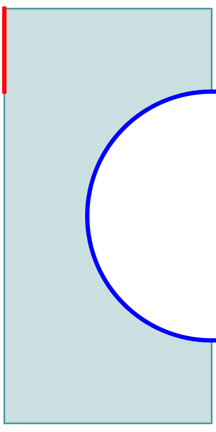
Poisson’s equation
Poisson’s equation
Setup
Ω=ImplicitRegion[0≤x≤5&&0≤y≤10&&!((x-5)^2+(y-5)^2≤3^2),{x,y}];op=-Laplacian[u[x,y],{x,y}]-20;
hu=ron∂
Γ
D
In[]:=
Γ
D
n
Γ
N
In[]:=
Γ
N
2
(x-5)
2
(y-5)
2
3
Solve:
In[]:=
uif=NDSolveValue[{op,},u,{x,y}∈Ω];
Γ
N
Γ
D
Out[]=

Boundary
Boundary
Default
How To Set Up:
How To Set Up:
◼
Geometry/Mesh
◼
PDEs
◼
Boundary Conditions
Heat sink
Heat sink
Ω
PDE
Heat sink
Heat sink
Γ
Heat sink
Heat sink
Solve
Visualize
Solid Mechanics
Solid Mechanics
Crankshaft held fixed at both ends, forces from the pistons deform the object.
Mesh
PDE parameters
PDE
Solve:
Visualize:
How To Set Up:
How To Set Up:
◼
Geometry/Mesh
◼
PDEs
◼
Boundary Conditions
Geometry/Mesh
Geometry/Mesh
◼
Import: STEP, stl, dxf, ...
◼
Create your own
OpenCascadeLink
OpenCascadeLink
◼
Link to OpenCascade CAD engine
OpenCascadeLink
OpenCascadeLink
Load OpenCascadeLink:
Convert a Ball to an OpenCascadeShape:
Inspect the type of the object:
Convert to a mesh:
Visualize the mesh:
OpenCascadeLink Supports
OpenCascadeLink Supports
OpenCascadeLink
OpenCascadeLink
Mesh Generation
Mesh Generation
Manual
Manual
Symbolic Regions
Symbolic Regions
Create the region product of a 2D mesh with a coarse 1D mesh.
Graded Meshes
Graded Meshes
Construct a region product.
Visualize the region product of the anisotropic mesh.
Multi-materials
Multi-materials
PMLs, Images, Contours,
PMLs, Images, Contours,
Mesh Generation
Mesh Generation
Mesh Generation
Mesh Generation
PDEs/BCs with Material Regions
PDEs/BCs with Material Regions
Shielded micro strip
Shielded micro strip
Ω
Shielded micro strip
Shielded micro strip
PDE
Γ
Shielded micro strip
Shielded micro strip
Solve
Visualize
Automation
Automation
Solvers
Solvers
◼
Linear/Nonlinear Stationary (both iterative/direct)
◼
Transient
◼
Frequency
◼
Parametric
◼
Eigenvalues
Transient
Transient
Transient
Transient
Transient
Transient
Eigenvalue Problem
Eigenvalue Problem
NDEigensystem
NDEigensystem
NDEigensystem
NDEigensystem
NDEigensystem
NDEigensystem
Mask tool boundary graphics :
NDEigensystem
NDEigensystem
NDEigensystem
NDEigensystem
NDSolve rocks!
NDSolve rocks!
Summary:
non-linear, variable coefficient, transient systems of PDEs over arbitrary regions in
1D/2D/3D
1D/2D/3D
Thanks
Thanks
Wave equation
Wave equation
POVRay rendering
Ca. 50K Elements, compute time ca. 5min, render time ca. 5 hours.
Specific PDEs
Specific PDEs
NeumannValues
NeumannValues
In this case, the generalized Neumann conditions are
FEM derivation:
Integration by parts gives:
If NeumannValue[-1,x5] floats around in the list of equations, we do not know with which equation to associate it!
Init
Init
CITE THIS NOTEBOOK
CITE THIS NOTEBOOK
Wolfram R&D LIVE: PDE Modeling
by Oliver Ruebenkoenig
Wolfram Community, STAFF PICKS, February 3 2023
https://community.wolfram.com/groups/-/m/t/2823264
by Oliver Ruebenkoenig
Wolfram Community, STAFF PICKS, February 3 2023
https://community.wolfram.com/groups/-/m/t/2823264