Wolfram Cloud Document

ABSTRACT (original article): Consider a distribution with several parameters whose exact values are unknown and need to be estimated using the maximum-likelihood technique. Under a regular case of estimation, it is fairly routine to construct a confidence region for all such parameters, based on the natural logarithm of the corresponding likelihood function. In this article, we investigate the case of doing this for only some of these parameters, assuming that the remaining (so called nuisance) parameters are of no interest to us. This is to be done at a chosen level of confidence, maintaining the usual accuracy of this procedure (resulting in about 1% error for samples of size , and further decreasing with 1/n). We provide a general solution to this problem, demonstrating it by many explicit examples. CITATION (original article): Vrbik, J. (2022), Confidence Regions with Nuisance Parameters. Open Journal of Statistics, 12, 658-675. https://doi.org/10.4236/ojs.2022.125039

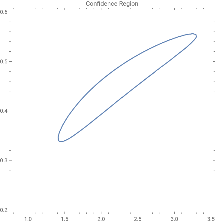
Assuming a sample of size n from a K-parameter distribution, we know that the difference between the natural logarithm of the square of the likelihood function evaluated using maximum likelihood estimators of K parameters, and evaluated using their true values has a chi-square distribution with K degrees of freedom. This can be used to construct the corresponding K dimensional confidence region for the parameters, as demonstrated by the following example. Note that in all our examples, the sample itself is generated randomly using Mathematica.

In[]:=

X=RandomVariate[NegativeBinomialDistribution[1.7,0.4],200];(*generatingasample*)lnf[x_]:=xLog[1-p]+αLog[p]+LogGamma[x+α]-LogGamma[α]-LogGamma[x+1](*lnofPMF*)lnLF=Apply[Plus,Map[lnf,X]]//Together;(*lnoflikelihoodfunction*)res=NMaximize[{lnLF,α>0,0<p<1},{α,p}];Print["MLEs:",res[[2]]](*findingMLEsofthetwoparametersbymaximizinglnLF*)c=InverseCDF[ChiSquareDistribution[2],0.90];(*criticalvaluefor90%confidenceregion*)ContourPlot[2(res[[1]]-lnLF)==c,{α,0.8,3.5},{p,0.2,0.6},PlotLabel->"Confidence Region"]

MLEs:{α2.10084,p0.439429}

Out[]=

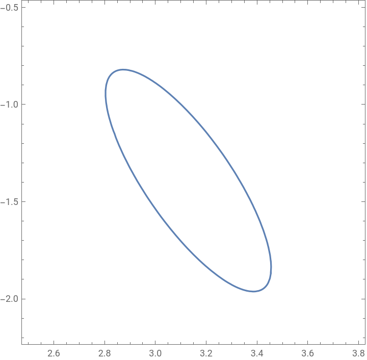
Similarly, when some parameter estimators (here, we consider ML estimators only) are asymptotically independent of all the remaining ones (called nuisance parameters), the same thing is true for the difference between

ln(

ℒ

) when evaluated with ML estimates of all parameters, and the same expression evaluated with true values of the parameters whose confidence region is to be constructed, while the remaining parameters remain at the same ML estimates. This is demonstrated in the next example using a sample from bivariate Normal distribution and finding a confidence region for the two means (considering the remaining three to be nuisance parameters); the second part of the example does the reverse.

X=RandomVariate[MultinormalDistribution[{3.2,-1.6},{{2.3,-2.9},{-2.9,6.2}}],120];(*randomsampleof120*)lnf[x_]:=-

(x[[1]]-

)



(x[[2]]-

)



-2ρ(x[[1]]-

)(x[[2]]-

)



2(1-

)-Log2π(1-

)

(*lnofNormalPDF*)lnLF=Apply[Plus,Map[lnf,X]]//Together;(*lnoflikelihoodfunction*)res=NMaximize[{lnLF,

>0,

>0,-1<ρ<1},{

,ρ}];Print["MLEs:",res[[2]]](*maximizelnLF*)aux1=lnLF/.res[[2,{3,4,5}]];(*leaveμ₁andμ₂unevaluated*)ContourPlot[2res[[1]]-2aux1==InverseCDF[ChiSquareDistribution[2],0.95],{

,2.5,3.8},{

,-2.2,-0.5}]aux2=lnLF/.res[[2,{1,2}]];(*leaveσ₁,σ₂ρunevaluated*)ContourPlot3D[2res[[1]]-2aux2==InverseCDF[ChiSquareDistribution[3],0.9],{

,1,2},{

,2,3},{ρ,-.9,-0.6}]

MLEs:{

3.12959,

-1.39143,

1.46021,

2.55678,ρ-0.785006}

Out[]=

In general, when the parameters of interest are not asymptotically independent of the nuisance parameters, things become more complicated. In the case of two parameters (one of them nuisance), the difference between the two

ln(

ℒ

) has now a chi-squared distribution with one degree of freedom, but further divided by

, where ρ is the asymptotic correlation coefficient between the two ML estimators. In our example, we find a confidence interval for the first parameter of a Gamma distribution (denoted α), ignoring the second (nuisance) parameter. In this case, the corresponding ρ is equal to the reciprocal of the square root of α PolyGamma[1,α]; note that it needs to be evaluated using the MLE of α.

X=RandomVariate[GammaDistribution[2.3,7.1],150];(*sampleof150*)lnf[x_]:=(α-1)Log[x]-x/β-LogGamma[α]-αLog[β];lnL=Apply[Plus,lnf[X]];res=NMaximize[{lnL,α>0,β>0},{α,β}];Print["MLEs: ",res[[2]]]aux=αPolyGamma[1,α]/.res[[2]];NSolve[2res[[1]]-2(lnL/.res[[2,2]])==InverseCDF[ChiSquareDistribution[1],0.90]/(1-1/aux),α,Reals];Print["90% CI for α: (",(α/.%[[1]]),", ",(α/.%[[2]]),")"]

MLEs: {α1.95742,β7.53034}

90% CI for α: (1.62558, 2.31476)

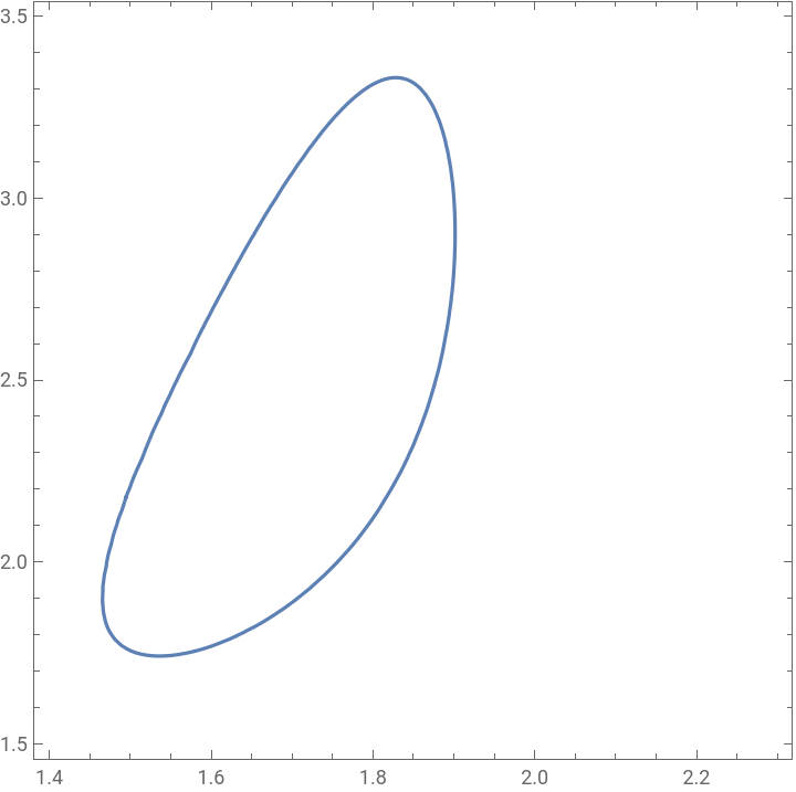
The case of three parameters is similar to the previous situation when only one of them needs to be estimated, while the other two are nuisance parameters. But reversing it (estimating the first two of three parameters), things get more complicated. To start with, we need to find the asymptotic correlation matrix of all three parameters and invert it; the first main-diagonal element of the last matrix (which corresponds to the nuisance parameter) is denoted s. The difference between the two

ln(

ℒ

) has now a more complicated PDF (f of the following program) involving a Bessel function and having s as its only parameter. The critical value (for a given level of confidence) can this time be found only numerically. As an example, we use a three-parameter Gamma distribution.

In[]:=

X=RandomVariate[GammaDistribution[0.32/2.6,1.8,2.6,0],1000];lnf[x_]:=-αLog[β]+Log[γ]-

+(α-1)Log[x]-LogGamma

lnLF=Apply[Plus,Map[lnf,X]]//Together;res=NMaximize[{lnLF,α>0,β>0,γ>0},{α,β,γ}];Print["MLEs: ",res[[2]]];aux=lnLF/.res[[2,1]];s=

α+γ

γ(α+γ)-

PolyGamma1,



+PolyGamma1,



PolyGamma1,



/.res[[2]];f=Exp-

s+1

yBesselI0,

s-1

y2

;c=c/.FindRoot[Integrate[f,{y,0,c}]==0.95,{c,4}];ContourPlot[2(res[[1]]-aux)==c,{β,1.4,2.3},{γ,1.5,3.5}]

MLEs: {α0.325946,β1.68126,γ2.37518}

Out[]=

Not surprisingly, the case of four parameters becomes more challenging yet; here we consider the case of constructing a confidence region for the last two parameters (the first two being nuisance parameters). We start by computing the variance-covariance matrix of all four parameters and its inverse, we then take the lower-right 2 by 2 corner of each, multiply the two and find the eigenvalues (denoted

and

) of the resulting matrix. The PDF of the

ln(

ℒ

)

difference involves the same Bessel function and both

and

as parameters. We demonstrate the technique using a mixture of Exponential and Normal distributions, constructing a confidence region for the two parameters of the Normal distribution, considering the other two (the weight and mean of the Exponential distribution) to be nuisance parameters.

In[]:=

aux=RandomVariate[BinomialDistribution[450,.4],1][[1]];(*0.4istheweightgiventoExponentialdistribution*)X=Join[RandomVariate[ExponentialDistribution[1/3.1],aux],RandomVariate[NormalDistribution[14.2,2.9],450-aux]];lnf[x_]:=LogaExp[-x/b]b+(1-a)Exp-

(x-c)

2



2Pi

dlnLF=Apply[Plus,Map[lnf,X]];res=NMaximize[{lnLF,b>0.1,0.1<a<0.9,d>0.1},{a,b,c,d}];Print["MLEs: ",res[[2]]]aux={D[lnf[x],a],D[lnf[x],b],D[lnf[x],c],D[lnf[x],d]};M=NIntegrate[Outer[Times,aux,aux]Exp[lnf[x]]/.res[[2]],{x,0,∞}];(*asymptoticV-Cmatrix*)t=Eigenvalues[M[[{3,4},{3,4}]].Inverse[M][[{3,4},{3,4}]]];z=Z/.FindRoot

t[[1]]t[[2]]/4

Integrate[Exp[-(t[[1]]+t[[2]])/4y]BesselI[0,(t[[1]]-t[[2]])/4y],{y,0,Z}]==0.9,{Z,4.};ContourPlot[2(res[[1]]-lnLF/.res[[2,{1,2}]])==z,{c,13,15},{d,2.5,3.4}]

The true value of α is thus, in this particular case, almost 6%, compared with the intended value of 5%. But we have deliberately selected both ρ and n to represent what can be considered a worse-case scenario; for larger samples and most other circumstances, the actual error can be expected to be a lot smaller.

CITE THIS NOTEBOOK

Confidence regions with nuisance parameters
by Jan Vrbik
Wolfram Community, STAFF PICKS, March 16, 2024
https://community.wolfram.com/groups/-/m/t/3141897