Hi fellow number geeks,
I am showing here how to determine the proportion of numbers in certain intervals whose prime factorisation is made up of a given total number of factors by using closed form expressions of the prime pi function with WL.
Enjoy,
Fabian
I am showing here how to determine the proportion of numbers in certain intervals whose prime factorisation is made up of a given total number of factors by using closed form expressions of the prime pi function with WL.
Enjoy,
Fabian
Prime Time
Prime Time
Prime numbers are distinguished by having exactly two natural numbers as dividers without remainder. This excludes 1 from being prime. The first 100 primes can be listed as
In[]:=
Prime[Range[100]]
Out[]=
{2,3,5,7,11,13,17,19,23,29,31,37,41,43,47,53,59,61,67,71,73,79,83,89,97,101,103,107,109,113,127,131,137,139,149,151,157,163,167,173,179,181,191,193,197,199,211,223,227,229,233,239,241,251,257,263,269,271,277,281,283,293,307,311,313,317,331,337,347,349,353,359,367,373,379,383,389,397,401,409,419,421,431,433,439,443,449,457,461,463,467,479,487,491,499,503,509,521,523,541}
The Greeks have given us formidable insight that there cannot be a largest prime number. That assumptions can be invalidated simply by forming the number consisting of the multiplication of such a finite set and then adding 1 which gives a new number having no divisor in that original set resulting in a contradiction with the assumption of a limited number of primes.
However we can guess from the list above that primes become increasingly rare the larger they get so that the search for the largest prime becomes something of a sport for large computers farms.
The prime counting function is defined as returning the number of primes smaller or equal to M. If we plot this function up to 500 we get the following graph illustrating the growth of the set of prime numbers.
π(M)
In[]:=
Plot[PrimePi[M],{M,0,500},PlotTheme"Detailed"]
Out[]=
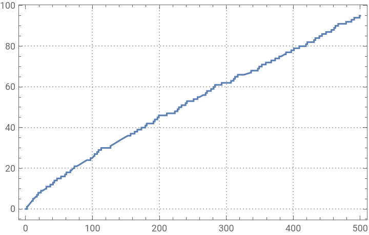

In order to read a result in such a plot you draw a vertical line at the number you are interested in to the intersection with the curve and then draw a horizontal line to read on the vertical axis the number that tells you the result, so π(400) is somewhere around a 80. Such a graph illustrates the connection between input and output of the prime pi function.
We see that has some regular evolution but we can also notice some randomness and intervals where it seems to stagnate for a while. Indeed the smooth or asymptotic behaviour of this curve has been described mathematically in the 19th century as
π(M)
In[]:=
Asymptotic[PrimePi[M],M∞]
Out[]=
M
Log[M]
This means that the proportion of prime numbers up to M is indeed vanishing as the inverse logarithm which explains that it becomes increasingly harder to break the world record for the largest verified prime without advancing computational power accordingly.
Many facets of prime numbers such as special algebraic forms of pairs of primes have interested mathematicians for ages but here we want to direct our attention to a fact that is telling us something about natural numbers in general. We start with the observation that any natural number can be written in a unique way as the multiplication of its prime factors, also called the integer factorization of the number, so or or in full algebraic generality
10=2×5
48=2×2×2×2×3
x=××…×,∈,<<…<
m
1
p
1
m
2
p
2
m
r
p
r
p
i
p
1
p
2
p
r
This defines a general unique way to write a natural number as a multiplication of increasing primes. The doublestruck P symbol is used here to denote the set of prime numbers.
So now let us now formulate the question which we would like to examine in some detail in the remainder. What is the distribution of natural numbers in a certain interval if we group them by the total number of prime factors = ++…+ of their factorization.
n
m
1
m
2
m
r
A mathematical expression for this counting function can be found if we assume that we include the interval of numbers larger than M and smaller or equal to 2M and sort out those with a total of n prime factors in the prime decomposition as follows:
PiC[n_,M_]:=≤∈,=2≤∈,=≤∈,=...≤...∈,=PrimePi...-PrimePiMax...,Max[q∈:q<,1]
p
1
n
2M
∑
p
1
p
1
p
2
n-1
2M
p
1
∑
p
2
p
2
p
1
p
3
n-2
2M
p
1
p
2
∑
p
3
p
3
p
2
p
n-1
2
2M
p
1
p
n-2
∑
p
n-1
p
n-1
p
n-2
2M
p
1
p
2
p
n-1
M
p
1
p
2
p
n-1
p
n-1
So let’s describe this somewhat convoluted expression. It consists of sums that index the primes in such a way that their combined product is less than and so that each subsequent one is at least as large as the previous one. The first of these starts from the initial prime number . Then in the summed terms we have the difference of the prime number counts in the interval scaled back from by subsequent divisions of prime numbers in the summation set. There is a slightly finicky exception to be made when the lower boundary of the interval becomes less than the increasing sequence of primes which we need to avoid by taking the maximum of arguments indicated there.
n-1
2M
2
M
If you are interested in further technicalities you also need to know that this expression is only correct if .
M>
n
2
The code corresponding to the first few orders of gives reasonably manageable expressions:
n
In[]:=
PiC[1,M_]:=PrimePi[2M]-PrimePi[M]
In[]:=
PiC[2,M_]:=Sum[PrimePi[2M/p]-PrimePi[Max[M/p,Prime[Max[1,PrimePi[p]-1]]]],p,Prime@Range@PrimePi@
2M
]In[]:=
PiC[3,M_]:=SumPrimePi[2M/p/q]-PrimePi[Max[M/p/q,Prime[Max[1,PrimePi[q]-1]]]],p,Prime@Range@PrimePi@,q,Prime@RangePrimePi[p],PrimePi
1
3
(2M)
2M/p
In[]:=
PiC[4,M_]:=SumPrimePi[2M/p1/p2/p3]-PrimePi[Max[M/p1/p2/p3,Prime[Max[1,PrimePi[p3]-1]]]],p1,Prime@Range@PrimePi@
4
2M
,p2,Prime@RangePrimePi[p1],PrimePi3
2M/p1
,p3,Prime@RangePrimePi[p2],PrimePi2M/p1/p2
Equipped with that code we are ready to make a plot illustrating the proportion of numbers with a prime factor count of 1, 2, 3 and 4 in the interval with varying from to
M+1...2M
M
16
10000
In[]:=
Mmin=16;Mmax=10000;stack={Table[{M,PiC[1,M]/M},{M,Mmin,Mmax}],Table[{M,PiC[2,M]/M},{M,Mmin,Mmax}],Table[{M,PiC[3,M]/M},{M,Mmin,Mmax}],Table[{M,PiC[4,M]/M},{M,Mmin,Mmax}]};
In[]:=
StackedListPlot[stack,ScalingFunctions{"Log10",None},PlotTheme"Detailed"]
Out[]=
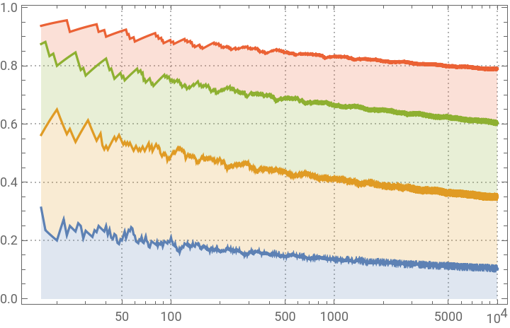
We see that with increasing M the proportion of numbers that contain a higher number of prime factors increases. This makes sense as we can rationalize from the fact that the logarithm function gives the typical number of factors needed to build up a target number by multiplication. We can always find an M large enough such that a majority of the numbers has more prime factors than any given fixed number n. Indeed knowing the distribution of the integer factorization proportions for a sufficiently large interval pins down that interval pretty well. Hence we have an interesting coupling between a statistical feature of integer factorization statistics and the magnitude of the numbers that generate it.
Hopefully you start to feel an itch to open a classic text or just the Wikipedia pages on number theory to learn with more rigor or with a broader view about the secret life of numbers. Even grander if you use the computational tools or code included here to fiddle around with other questions that might stir your interest.