A tensor network is a graph annotated with tensors and contraction indices. A quantum circuit can be understood as a tensor network, where each gate is replaced by corresponding tensor, and edges represents corresponding index contractions. In this short computational essay, we explore tensor networks in the Wolfram quantum framework, and discuss how it provides a more efficient way to do computations.
Wolfram Quantum Team (quantum AT wolfram.com)
Paclet installation
Paclet installation
Install Wolfram quantum paclet:
In[]:=
PacletInstall["Wolfram/QuantumFramework"]Needs["Wolfram`QuantumFramework`"]
Out[]=
PacletObject

One can also use the developer link to install the paclet; which is updated more often (eg daily) compared to the paclet link above:
PacletInstall["https://wolfr.am/DevWQCF",ForceVersionInstall->True]
Tensor networks
Tensor networks
Create a quantum circuit:
In[]:=
circuit=QuantumCircuitOperator[{"S","H"->2,"X"->3,"CNOT","SWAP"->{2,3},{1},{2},{3}}];circuit["Diagram"]
Out[]=
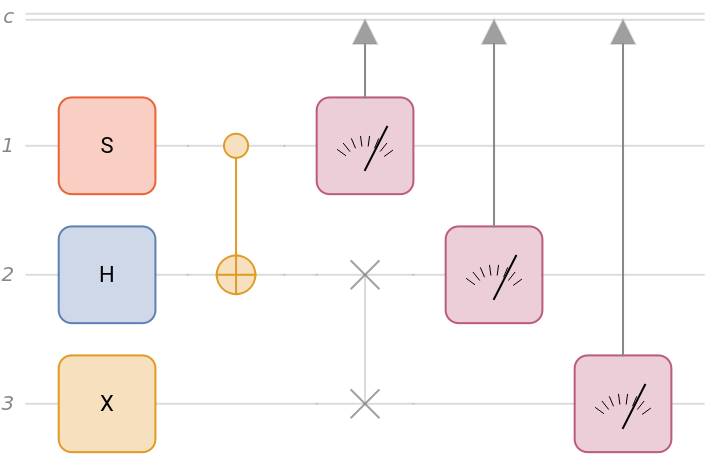
Note in Wolfram quantum framework, each measurement result is saved in an ancillary quantum system (call it a detector, for example). So the true diagram will be something like this:
In[]:=
circuit["Diagram","ShowExtraQudits"->True]
Out[]=
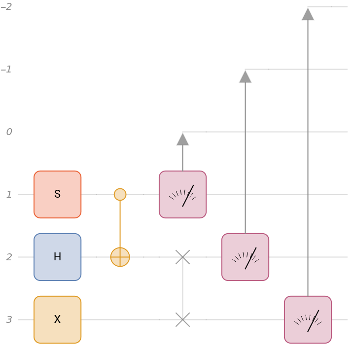
Note the first measurement is saved in the wire labeled as 0 and the rest goes backward, with negative labels.
Return the tensor network representation of the circuit:
In[]:=
net=circuit["TensorNetwork",GraphLayout->{"LayeredDigraphEmbedding","Orientation"->Left}]
Out[]=
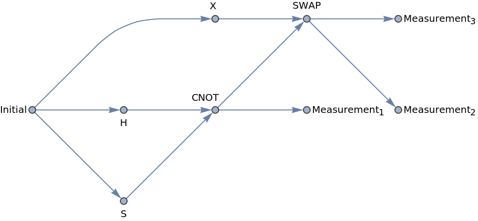
The tensor network is a graph annotated with tensors and contraction indices.
In[]:=
GraphQ[net]&&TensorNetworkQ[net]
Out[]=
True
Lists all annotation keys available for the tensor network:
In[]:=
AnnotationKeys[{net,0}]
Out[]=
{Index,Tensor,VertexCoordinates,VertexLabels,VertexShape,VertexShapeFunction,VertexSize,VertexStyle}
Let’s look at tensor, vertex labels, and corresponding indexes in the tensor network:
In[]:=
list=Developer`FromPackedArray@VertexList[net];TableFormTranspose[Prepend[AnnotationValue[{net,list},#]&/@{"Tensor","Index"},Sort@AnnotationValue[net,VertexLabels]]],
Out[]//TableForm=
VertexLabel | Tensor | Index |
0Initial | SparseArray | { 1 0 2 0 3 0 |
1S | SparseArray | { 1 1 1 1 |
2H | SparseArray | { 2 2 2 2 |
3X | SparseArray | 3 3 3 3 |
4CNOT | SparseArray | { 1 4 2 4 4 1 4 2 |
5SWAP | SparseArray | 2 5 3 5 5 2 5 3 |
6 Measurement 1 | SparseArray | { 0 6 1 6 6 1 |
7 Measurement 2 | SparseArray | { -1 7 2 7 7 2 |
8 Measurement 3 | SparseArray | -2 8 3 8 8 3 |


Note tensors in the tensor network are mixed type, meaning they consist of so-called “contravariant” (upper) indices and “covariant” (lower) indices. For example, the 2nd measurement (7th vertex), acts on qubit-2 (denoted by contravariant and covariant indices 2) and its result is saved on wire, denoted by the index “-1”.
Vertices correspond to circuit’s operators/gate indices, in addition to “Initial” tensor with index 0 (for the initial state):
In[]:=
VertexList[net]
Out[]=
{0,1,2,3,4,5,6,7,8}
In[]:=
Length@circuit["Flatten"]["Operators"]
Out[]=
8
In[]:=
%==Max[%%]
Out[]=
True
Note that each edge represents (i.e., is tagged by) a contraction:
In[]:=
EdgeList[net]
Out[]=
01,02,03,14,24,45,35,46,57,58
,
1
0
1
1
,
2
0
2
2
,
3
0
3
3
,
1
1
4
1
,
2
2
4
2
,
2
4
5
2
,
3
3
5
3
,
1
4
6
1
,
2
5
7
2
,
3
5
8
3
Perform the contraction:
In[]:=
finalTensor=ContractTensorNetwork[net]
Out[]=
SparseArray
Confirm that the result is the same as default circuit application:
In[]:=
circuit[]["Tensor"]==finalTensor
Out[]=
True
Another tensor network representation uses indices as graph vertices with tensors as cliques:
In[]:=
indexNet=TensorNetworkIndexGraph[net,GraphLayout->{"LayeredDigraphEmbedding","Orientation"->Left}]
Out[]=
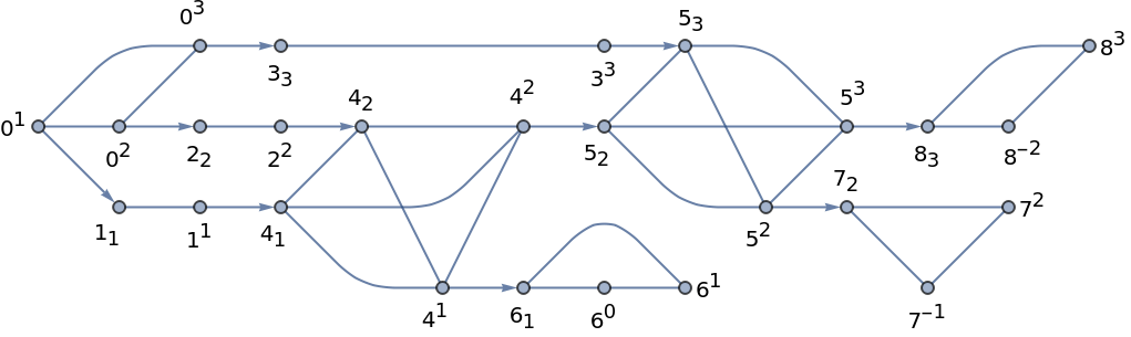
Note in above graph, the directed edges imply tensor contraction; also tensors are cliques in above graph
Free indices are the ones that left after contraction:
Free indices can be extracted as vertices with zero in- and out- degree:
Contraction and Einstein Summation
Contraction and Einstein Summation
What ContractTensorNetwork does is in fact EinsteinSummation.
Show ContractTensorNetwork is the same as EinsteinSummation:
One can compare the performance, on how the relevant computation is done
Perform the contraction in the order of network’s EdgeList:
Optimize the order for contraction, using EinsteinSummation and symbolic tensors package:
Initial state different from ground state
Initial state different from ground state
Note that the initial tensor in the tensor network we studied here was a registered state. Additionally, one can start from any initial state.
Generate a random state:
Initialize the tensor network from above state:
See supplement info, for package-scoped symbols.
Show the tensor contraction is the same as transformation of state by the circuit:
Supplement info
Supplement info
CITE THIS NOTEBOOK
CITE THIS NOTEBOOK
Tensor networks and quantum computation
by Mads Bahrami
Wolfram Community, STAFF PICKS, July 25, 2023
https://community.wolfram.com/groups/-/m/t/2976463
by Mads Bahrami
Wolfram Community, STAFF PICKS, July 25, 2023
https://community.wolfram.com/groups/-/m/t/2976463