Introduction
Introduction
Before I talk about the subject of this essay, I would like to make a couple of points. Firstly, I was inspired to write this by the fantastic book ‘Classical Mechanics: the Theoretical Minimum’ by Leonard Susskind and George Hrabovsky, which was my first introduction to multivariable calculus. I would thoroughly recommend it to anyone who wishes to learn more about mathematics and physics (which the book considers at a low undergraduate level, I believe). I myself do not have undergraduate knowledge of the topic, so this essay is essentially my own personal Beginner’s Guide to Multivariable Calculus.
The aim of this is therefore more of a computational lecture, as it were, which I have designed to introduce the idea of 3-dimensional plots, maxima, minima and saddle points, assisted by the Wolfram Language. We will be considering things such as Hessian matrices, partial derivatives, etcetera. For that reason I doubt this will be of interest to a large number of people, but hopefully it does provide some help for anyone new to this subject.
The aim of this is therefore more of a computational lecture, as it were, which I have designed to introduce the idea of 3-dimensional plots, maxima, minima and saddle points, assisted by the Wolfram Language. We will be considering things such as Hessian matrices, partial derivatives, etcetera. For that reason I doubt this will be of interest to a large number of people, but hopefully it does provide some help for anyone new to this subject.
3-Dimensional Plots in the Wolfram Language
3-Dimensional Plots in the Wolfram Language
3D visualisation is very simple in the Wolfram Language, although the function you use will depend on what you are plotting (e.g. a surface, a curve). But firstly we need to consider the 3D space. You will, I hope, be familiar with the idea of the x-, y- and z-axes. Now, forget about the z-axis for the moment, and consider a 2D plot, say It’s best here to really examine what this actually is: the function is f, the output is f(x), and the input is x, which for this we can just assume belongs to the set of Real numbers.Now, our input x is a variable, being that we can change the value to get a different output. It may be tempting to think of the output f(x) as a variable, because it changes - but it’s important to realise that it changes only because x does. Therefore this is a function with only one variable. It is worth noting that, of course, we plot the output on the y-axis, and the corresponding input on the x-axis (although of course this depends on what we called that variable in the first place).Now, assume we have a function f(x, . Here we can see we have two input variables - x and y. So the result of f(x, y) is going to be dependent on both of them - the value of f(x, y) will be different between if x=2 and y=3, and if x=2 and y=4: even though the x-input has stayed the same. Now, we can plot this using Mathematica’s function 3DPlot: which is exceedingly useful, because more complicated 3D graphs can be incredibly hard to visualise.
f(x)=.
2
x
y)=+
2
x
2
y
Where -10 ≤ x ≤ 10, and -10 ≤ y ≤ 10.
In[]:=
Plot3D[x^2+y^2,{x,-10,10},{y,-10,10}]
Out[]=
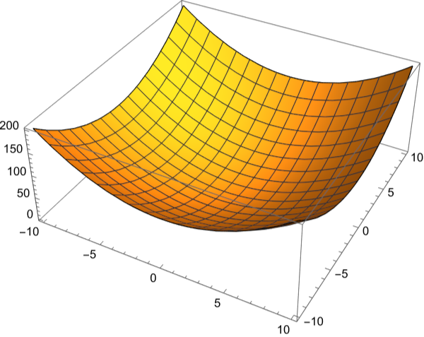
Handily, Mathematica wraps our graph up in a nice cuboid, allowing us to see the boundaries easily. The two base-axes are x and y, and the side-axis is f(x,y), which we could in theory call z by replacing our f(x) with it. We can draw some nice parallels between this and a quadratic equation in 2 dimensions: there is only one minimum point, and from there the graph ‘rises’ uniformly.
Maxima, Minima and Saddle Points
Maxima, Minima and Saddle Points
Now that we’ve had our first look at 3D plots and multivariable functions, let’s consider the actual calculus that awaits. Differentiation, of course, is just the rate of change, and it therefore plays a major part in practically all of mechanics (and more). Some really important points in any graph (perhaps it would be better to refer to it as a model) are when the rate of change hits zero. This often signifies something major, and is very useful in numerous fields. There are 3 main ‘stationary’ points: maxima, minima, and saddle points.
Consider the former, which is quite self-explanatory. It refers to when a model reaches a maximum point. At this point the rate of change is zero, because the curve of the entire graph changes from going up (with a positive gradient) to going down (with a negative gradient). Depending on the function, we could see multiple maxima, because the graph could peak at multiple points. Local maxima are the points where this happens in a region, and so we can have any number of these. However, the Global maximum is the largest value (or output) for f(x,y) across every value of x and y: were we to see it in a plot, there would be no other point higher than it.
Minima are effectively the opposite, and can also be local or global. At a minimum point the gradient changes from negative to positive on either side. You can see this in our 3DPlot up above, where the graph dips inwards until it meets at the point (0,0). In that case (0,0) is the site of the global minimum point, because it is the lowest point in the graph.
Saddle Points are (by definition as a stationary point) also where the gradient is 0. However, they are not extremum, or in other words while it will curve up in one direction it will curve down in the other direction, like a saddle - whereas, if we assume that it is instead a maximum, in all directions it will curve downward.
Now we have considered all these points, how can we find them on a graph? For a 2D graph (excluding saddle points, which we can in theory replace with ‘inflection’ points: however inflection points mean that the function changes from concave to convex, or vice versa, so we’ll ignore them) we would find the derivative and set this equal to 0. For example the derivative of is 4x + 4 (multiply by the power, decrease the power by 1). When 4x+4=0, x is equal to -1, so the graph has a minimum (being that it’s a quadratic with a positive coefficient of ) at (-1, -2), getting the output using the original function. If we plot this, we should see precisely that:
Consider the former, which is quite self-explanatory. It refers to when a model reaches a maximum point. At this point the rate of change is zero, because the curve of the entire graph changes from going up (with a positive gradient) to going down (with a negative gradient). Depending on the function, we could see multiple maxima, because the graph could peak at multiple points. Local maxima are the points where this happens in a region, and so we can have any number of these. However, the Global maximum is the largest value (or output) for f(x,y) across every value of x and y: were we to see it in a plot, there would be no other point higher than it.
Minima are effectively the opposite, and can also be local or global. At a minimum point the gradient changes from negative to positive on either side. You can see this in our 3DPlot up above, where the graph dips inwards until it meets at the point (0,0). In that case (0,0) is the site of the global minimum point, because it is the lowest point in the graph.
Saddle Points are (by definition as a stationary point) also where the gradient is 0. However, they are not extremum, or in other words while it will curve up in one direction it will curve down in the other direction, like a saddle - whereas, if we assume that it is instead a maximum, in all directions it will curve downward.
Now we have considered all these points, how can we find them on a graph? For a 2D graph (excluding saddle points, which we can in theory replace with ‘inflection’ points: however inflection points mean that the function changes from concave to convex, or vice versa, so we’ll ignore them) we would find the derivative and set this equal to 0. For example the derivative of
2+4x
2
x
2
x
In[]:=
Plot[2x^2+4x,{x,-3,3}]
Out[]=
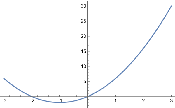
And from there we can use the second derivative to actually identify what these points are.
But, how do we do this for a function like f(x,y)? The answer is, of course, derivatives - but we have to use partial derivatives, with respect to each variable.
But, how do we do this for a function like f(x,y)? The answer is, of course, derivatives - but we have to use partial derivatives, with respect to each variable.
Partial Differentiation and Identifying Stationary Points
Partial Differentiation and Identifying Stationary Points
All we are doing for partial differentiation is doing differentiation but only with respect to one of the variables. Consider dy/dx as our standard form for differentiation, where y is our function, and x is what we are differentiating with respect to. What we are doing when differentiating can be seen from first principles: adding a minute change to x and seeing what happens to the gradient as the change tends to 0. In other words: = (f(x + Δx) - f(x)) / ΔxWhere the denominator simplifies to Δx (you might know this as the gradient being ) over (-)"). Note, of course that capital Delta just refers to a change: some prefer to simplify this to “h”. So, for a partial derivative, using our previous example of f(x,y), we can use (f(x+Δx,y)-f(x,y)) / ΔxDo remember that in this case we are finding the partial derivative with respect to x - if we wanted it with respect to y we’d just change the formula.The notation for this, incidentally, is:Something important to remember is that is not uncommon (indeed, it is more often than not) for us to still be left with the variable y. This can be seen for an equation like -5xy+3-10x+7y-22, because of that xy term that joins them together. The partial derivative of which is 2x-5y-10. This in itself is not the best plot to use for my future explanations, so instead I will switch to this simple but effective plot:
y
x
Δx->0
"(-
y
2
y
1
x
2
x
1
Δx->0
∂y
∂x
2
x
2
y
Where f(x,y) = sin(x)+sin(y).
In[]:=
Plot3D[Sin[x]+Sin[y],{x,-7,7},{y,-7,7}]
Out[]=
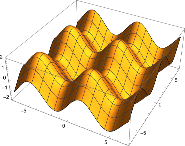
So, we know from before that the derivative of the function must be 0 for a point to be stationary. In multivariable calculus, we have to find the partial derivatives for every variable and then check that these are equal to 0 at the same point. Remember, of course, that these functions could have 3 variables: but the logic behind it is easily expandable.In this case, we can probably work out quite easily that:=cos(x)and=cos(y).We could work out when these are equal to 0 ourselves, but it’s much easier to use Mathematica:
∂f
∂x
∂f
∂y
In[]:=
Solve[Cos[x]==0,x,Assumptions->-7<x<7]
Out[]=
x-,x-,x,x
3π
2
π
2
π
2
3π
2
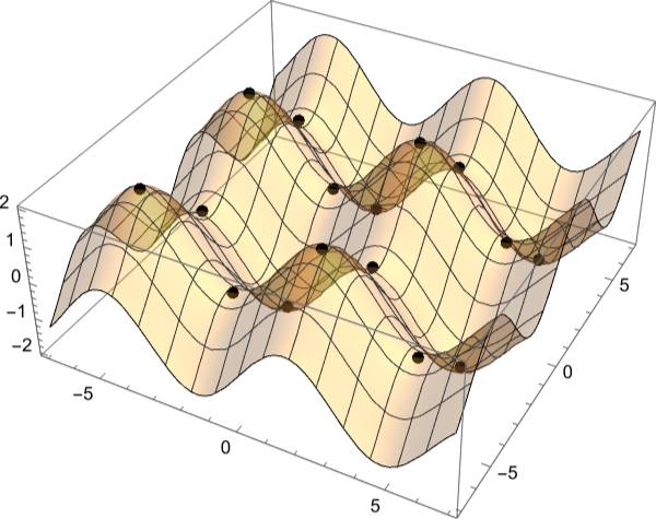
Of course giving us the right answers. Note, there are infinite solutions to this equation: we just have the ones between the limits of our variables. Now let’s plot them on our graph (and remember, we can plot this for both x and y, as they were the same function sine):
In[]:=
f=Sin[#1]+Sin[#2]&;a=Plot3D[Sin[x]+Sin[y],{x,-7,7},{y,-7,7},PlotStyle->Opacity[0.3]];xvalues=Solve[Cos[x]==0,x,Assumptions->-7<x<7];xvalues=Table[x/.xvalues[[a]][[1]],{a,1,Length[xvalues]}];yvalues=Solve[Cos[y]==0,y,Assumptions->-7<y<7];yvalues=Table[y/.yvalues[[b]][[1]],{b,1,Length[xvalues]}];zvalues=Level[Table[f[xvalues[[i]],yvalues[[j]]],{i,1,Length[xvalues]},{j,1,Length[yvalues]}],{2}];xandyvalues=Level[Table[{xvalues[[i]],yvalues[[j]]},{i,1,Length[xvalues]},{j,1,Length[yvalues]}],{2}];coordinates=Table[Append[xandyvalues[[i]],zvalues[[i]]],{i,1,Length[xandyvalues]}];b=ListPointPlot3D[coordinates,PlotStyle->Black];Show[a,b]
Out[]=
The above is probably the worst piece of code I have ever written, but it does the job. Let’s consider what it’s doing:
Firstly, I am creating a function to represent the function of our graph. I am then plotting this like usual, using a slightly lower opacity so I can see all of my stationary points. Later, I will also create a plot for these stationary points, and then merge the two together as my final act.
I am them solving to find where the derivative is 0 (as explained earlier), for both my x and y values. I could have just used the Wolfram Language’s Derivative function, but imagine that I have just done it mentally: also, remember that these are the second derivatives with respect to x and y, so if my function was in fact:
f(x,y) = cos(x)+sin(y)
I would instead be creating those tables for where the derivatives are equal to 0 by looking at cos(y) and -sin(x).
From here I used my function f to find the z values, but importantly here I am finding the z-values for all possible permutations of x and y (hence my nested loop). In this case, because my partial derivatives with respect to y and x are the same I can just find all the different orders, because they are equal at the same point.
It is a vital note here that, were our derivatives different, we would have to check that at each coordinate both partial derivatives are equal to 0 (which we explained earlier, also). This would easily be rememedied by a simple if-statement, thankfully.
And from there it’s just the plot, which we can see above, with the black dots showing our stationary points. We can see just by looking that we have 4 maximum points, 4 minimum and 8 saddle points in our region. Even so, it’s a bit hard to distinguish them - particularly those of the minima and saddles. Thankfully, there is a relatively simple way that we can find out what kind of stationary points these are.
Firstly, I am creating a function to represent the function of our graph. I am then plotting this like usual, using a slightly lower opacity so I can see all of my stationary points. Later, I will also create a plot for these stationary points, and then merge the two together as my final act.
I am them solving to find where the derivative is 0 (as explained earlier), for both my x and y values. I could have just used the Wolfram Language’s Derivative function, but imagine that I have just done it mentally: also, remember that these are the second derivatives with respect to x and y, so if my function was in fact:
f(x,y) = cos(x)+sin(y)
I would instead be creating those tables for where the derivatives are equal to 0 by looking at cos(y) and -sin(x).
From here I used my function f to find the z values, but importantly here I am finding the z-values for all possible permutations of x and y (hence my nested loop). In this case, because my partial derivatives with respect to y and x are the same I can just find all the different orders, because they are equal at the same point.
It is a vital note here that, were our derivatives different, we would have to check that at each coordinate both partial derivatives are equal to 0 (which we explained earlier, also). This would easily be rememedied by a simple if-statement, thankfully.
And from there it’s just the plot, which we can see above, with the black dots showing our stationary points. We can see just by looking that we have 4 maximum points, 4 minimum and 8 saddle points in our region. Even so, it’s a bit hard to distinguish them - particularly those of the minima and saddles. Thankfully, there is a relatively simple way that we can find out what kind of stationary points these are.
The Hessian Matrix and Identifying the Types of Stationary Points
The Hessian Matrix and Identifying the Types of Stationary Points
Short note: from here we are looking only at functions with 2 variables: it differs otherwise.If you have ever done calculus at a lower level (or if you remember my earlier statement), you probably remember that to find the type of stationary point for a point we need the second derivatives. The same applies for multivariable calculus - but we need all the second derivatives. The key point here is that we can find the second derivative with respect to x or y (or all our variables):forfHowever, we can also mix our variables for our second derivative: for example by differentiating with respect to x, but then differentiating with respect to y for the second derivative, giving us:forfWe would of course have more of these had we more variables. If you consider our own function that we plotted above, our mixed second derivatives will be zero, because after we differentiate with respect to either of our variables once, we are left only with that variable. The first thing we need to do when labelling stationary points is put these into the so-called Hessian Matrix, which looks like this:
2
∂
∂
2
x
2
∂
∂
2
y
2
∂
∂x∂y
2
∂
∂y∂x
For the sake of simplicity I won’t use the Wolfram Language’s capabilities to do a lot of the things it should do. But, I will use it to find all of our derivatives and second derivatives.
Note that Derivative and D are both derivative functions but work in slightly different ways.
From there, we can fill out our Hessian Matrix like so:
The next thing we need to know about are the Determinants and Traces: the former is likely to be more familiar with you. The Determinant, can be read as ad - bc for matrix:
And the Trace as a + d. Now, from here we have 3 rules (after substituting our points in):
If the Determinant and Trace are positive, the point is a (local) minimum.
If the Determinant is positive and the Trace negative, the point is a (local) maximum.
And finally, if the Determinant is negative (we can exclude the Trace if so), then the point is a saddle point. Let’s test it out, by pulling our coordinates of the stationary points we found earlier.
If the Determinant and Trace are positive, the point is a (local) minimum.
If the Determinant is positive and the Trace negative, the point is a (local) maximum.
And finally, if the Determinant is negative (we can exclude the Trace if so), then the point is a saddle point. Let’s test it out, by pulling our coordinates of the stationary points we found earlier.
And lo and behold, there we have it. Our points have been successfully colour-coded dependent on their type. You’ll see that again my code above is quite terrible, and not at all automated like it should really be - but I have done that on purpose so you can hopefully see what I’m doing.
Conclusion
Conclusion
This was very fun to write, and Mathematica (and such) is very useful for helping to visualise anything like this. The actual mathematics here isn’t very complicated whatsoever, but all the same hopefully this can be of use to anyone new to this, or to the Wolfram Language. Until the next time!
CITE THIS NOTEBOOK
CITE THIS NOTEBOOK
A beginner's guide to stationary points within multivariable functions
by Theo Vine
Wolfram Community, STAFF PICKS, October 29, 2024
https://community.wolfram.com/groups/-/m/t/3310829
by Theo Vine
Wolfram Community, STAFF PICKS, October 29, 2024
https://community.wolfram.com/groups/-/m/t/3310829