Adiabatic Reactors: Multiple Steady States
Authors: Housam Binous and Ahmed Bellagi
Adiabatic Reactors: Multiple Steady States
Authors: Housam Binous and Ahmed Bellagi
Authors: Housam Binous and Ahmed Bellagi
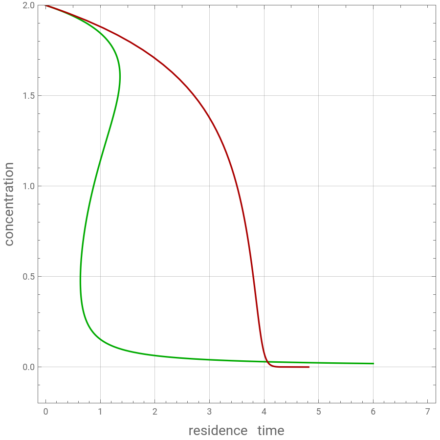
We plot the concentration and temperature versus residence time in an adiabatic Continuous Stirred Tank Reactor (CSTR) and an adiabatic plug flow tubular reactor (PFTR ).
Multiple steady states are obtained for the adiabatic CSTR case . In fact, for a residence time equal to one and the adiabatic CSTR case, three values of the concentrations are found . In addition, we find that the CSTR can require much smaller residence times than the PFTR .
Multiple steady states are obtained for the adiabatic CSTR case . In fact, for a residence time equal to one and the adiabatic CSTR case, three values of the concentrations are found . In addition, we find that the CSTR can require much smaller residence times than the PFTR .
Acknowledgement :
Numerical values were obtained from textbook of Lanny D. Schmidt, The Engineering of Chemical Reactions, Oxford University Press, 1998.
Numerical values were obtained from textbook of Lanny D. Schmidt, The Engineering of Chemical Reactions, Oxford University Press, 1998.
Relationship between temperature and concentration for an adiabatic CSTR and an adiabatic PFTR
In[]:=
Sol1=Solve[ρ(T-T0)+(-x)(-ΔH)0,T]//FullSimplify
c
p
C
A0
Out[]=
TT0+
ΔH(-x+)
C
A0
ρ
c
p
In[]:=
Sol2=Solve[(ρ(T-T0)+(-ΔH)(-x))0,x]
c
p
C
A0
Out[]=
x
-Tρ+T0ρ+ΔH
c
p
c
p
C
A0
ΔH
Numerical values
In[]:=
k
0
In[]:=
Ea=15000;
In[]:=
ΔH=20000;
In[]:=
T0=300;
In[]:=
ρ=1000/;
c
p
In[]:=
C
A0
Relationship between temperature and concentration for an adiabatic CSTR and an adiabatic PFTR
In[]:=
T[x_]:=First[T/.Sol1]
In[]:=
T[x]
Out[]=
300+20(2-x)
rate constant
In[]:=
k[x_]:=Exp[-Ea/T[x]]
k
0
In[]:=
k[x]
Out[]=
2.6×
20
10
-
15000
300+20(2-x)
reaction rate
In[]:=
r[x_]:=k[x] x
In[]:=
r[x]
Out[]=
2.6×x
20
10
-
15000
300+20(2-x)
Concentration versus residence time for an adiabatic CSTR
τ=-
C
A0
C
A
k
C
A
In[]:=
pp=Plot[(2-x)/r[x],{x,0,2.0},PlotRange->{0,6},PlotStyle->Darker@Green,AspectRatio1,ImageSize 450{1,1},
GridLinesAutomatic,FrameTrue];
GridLinesAutomatic,FrameTrue];
In[]:=
pp1=Show[pp/.x_LineMap[Reverse,x,{2}],FrameLabel {Style["residence time",14],Style["concentration",14]},PlotRange->{{0,4},{0,2.4}}]
Out[]=
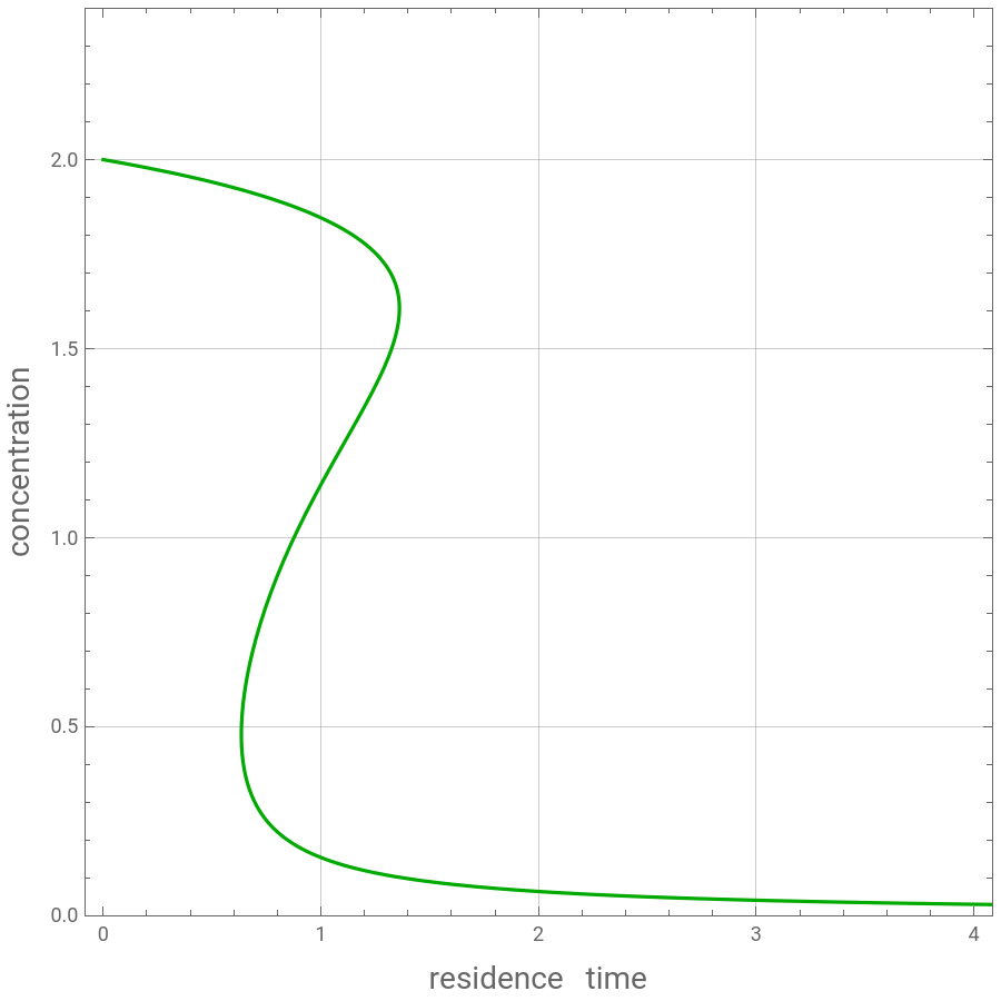
Concentration versus residence time for an adiabatic PFTR
τ=
1
k
C
A
C
A
In[]:=
τ[C_]:=NIntegrate[1/r[x],{x,2,C}]
In[]:=
kk=Plot[-τ[x],{x,0,2},PlotStyle->Darker@Red,AspectRatio1,ImageSize 450{1,1}, GridLinesAutomatic,FrameTrue];
In[]:=
kk1=Show[kk/.x_LineMap[Reverse,x,{2}],FrameLabel {Style["residence time",14],Style["concentration",14]},PlotRange->{{0,7},{0,2.4}}]
Out[]=
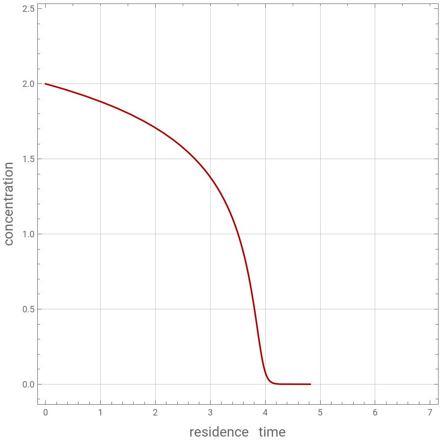
Concentration versus residence time for an adiabatic PFTR and an adiabatic CSTR. We find that the CSTR require much smaller residence times than the PFTR.
In[]:=
Show[pp1,kk1,PlotRange->{{0,7},{-0.2,2}}]
Out[]=
Relationship between concentration and temperature for an adiabatic CSTR and an adiabatic PFTR
In[]:=
x[T_]:=First[x/.Sol2]
In[]:=
x[T]
Out[]=
340000-1000T
20000
rate constant
reaction rate
In[]:=
r[T_]:= k[T] x[T]
Temperature versus residence time for an adiabatic CSTR
In[]:=
ll=Plot[(2-x[T])/r[T],{T,300,360},PlotStyle->Darker@Green,AspectRatio1,ImageSize 450{1,1}, GridLinesAutomatic,FrameTrue,PlotRange->All];
In[]:=
ll1=Show[ll/.x_LineMap[Reverse,x,{2}],FrameLabel {Style["residence time",14],Style["temperature",14]},PlotRange->{{0,5},{300,340}}]
Temperature versus residence time for an adiabatic PFTR
In[]:=
mm=Plot[NIntegrate[1/r[T] 1/20,{T,300,z}],{z,300,340},PlotStyle->Darker@Red,AspectRatio1,ImageSize 450{1,1}, GridLinesAutomatic,FrameTrue];
In[]:=
mm1=Show[mm/.x_LineMap[Reverse,x,{2}],FrameLabel {Style["residence time",14],Style["temperature",14]},PlotRange->{{0,7},{300,340}}]
Temperature versus residence time for an adiabatic PFTR and an adiabatic CSTR
In[]:=
Show[mm1,ll1,PlotRange->{{0,5},{300,340}}]
In[]:=
T[x_]:=First[T/.Sol1]
In[]:=
r[x_]:=k[x] x
In[]:=
jj=Plot[1/f,{x,0,1.99},PlotRange->{{0,2.4},{0,7}},Frame->True,GridLines->Automatic,
AspectRatio->1,ImageSize->350{1,1},FrameLabel {Style["CA0-CA",14],Style["1/r",14]}]
AspectRatio->1,ImageSize->350{1,1},FrameLabel {Style["CA0-CA",14],Style["1/r",14]}]
In an adiabatic CSTR, multiple steady states are obtained for example for a residence time equal to one.
Residence time is the colored area in the figures.
The same area is obtained for three different values of the concentration and temperature.
Conclusion: We obtain three steady states for certain values of the residence time in an adiabatic CSTR.
Residence time is the colored area in the figures.
The same area is obtained for three different values of the concentration and temperature.
Conclusion: We obtain three steady states for certain values of the residence time in an adiabatic CSTR.
In[]:=
Off[General::spell1]
In[]:=
sol1=FindRoot[f1,{ξ,0.1}]
In[]:=
sol2=FindRoot[f1,{ξ,1}]
In[]:=
sol3=FindRoot[f1,{ξ,2}]
In[]:=
plt1=Show[jj,Plot[g1,{u,0.0001,2-ξ}/.sol1,PlotRange->{{0,2.4},{0,7}},Frame->True,GridLines->Automatic,
AspectRatio->1,ImageSize->350{1,1},PlotStyle-> Darker@Red,FrameLabel {Style["CA0-CA",14],Style["1/r",14]},Filling->Axis]]
AspectRatio->1,ImageSize->350{1,1},PlotStyle-> Darker@Red,FrameLabel {Style["CA0-CA",14],Style["1/r",14]},Filling->Axis]]
In[]:=
plt1=Show[jj,Plot[g2,{u,0.0001,2-ξ}/.sol2,PlotRange->{{0,2.4},{0,7}},Frame->True,GridLines->Automatic,
AspectRatio->1,ImageSize->350{1,1},PlotStyle-> Darker@Green,FrameLabel {Style["CA0-CA",14],Style["1/r",14]},Filling->Axis]]
AspectRatio->1,ImageSize->350{1,1},PlotStyle-> Darker@Green,FrameLabel {Style["CA0-CA",14],Style["1/r",14]},Filling->Axis]]
In[]:=
plt1=Show[jj,Plot[g3,{u,0.0001,2-ξ}/.sol3,PlotRange->{{0,2.4},{0,7}},Frame->True,GridLines->Automatic,
AspectRatio->1,ImageSize->350{1,1},PlotStyle-> Darker@Cyan,FrameLabel {Style["CA0-CA",14],Style["1/r",14]},Filling->Axis]]
AspectRatio->1,ImageSize->350{1,1},PlotStyle-> Darker@Cyan,FrameLabel {Style["CA0-CA",14],Style["1/r",14]},Filling->Axis]]