Benford’s Law predicts the distribution of leading digits in many naturally occurring numerical data sets and some sequences. The convergence behavior of sequences satisfying Benford’s Law has been relatively unstudied. This project investigates which integer sequences exhibit Benford behavior and studies their convergence. New results establish conditions under which asymptotic Benford behavior is preserved under additive perturbations. We explored nestedly recursive sequences searching for Benford behavior but found none within this family. We quantified convergence toward the Benford distribution using total variation distance, with plots illustrating convergence and best fit functions. Fascinating total variation patterns were also found in sequences that do not satisfy Benford’s Law.
1) Introduction
1) Introduction
Benford’s Law describes the curious phenomenon that, in many naturally occurring sets of real numbers, the leading digit of terms is not uniformly distributed. Instead, smaller digits appear more frequently, with the digit 1 as the leading digit roughly 30% of the time. In fact, the probability that a digit d ∈ {1,2,…,9} appears as the leading digit can be described by the logarithmic distribution (1 + ). This surprising result (known as Benford’s Law) has been observed in a wide variety of contexts, including financial data, physical constants, city populations, and many mathematical sequences. While many individual sequences are widely known to satisfy Benford’s Law, comparatively little attention has been devoted towards the manner in which such sequences converge to the Benford distribution. This project aims to investigate the leading digit distribution behavior of several classes of positive integer sequences, with an emphasis on comparing patterns of convergence using total variation distance. We also aim to draw connections between sequences that do and do not exhibit Benford behavior. This notebook combines theoretical results with computational experiments. After deriving Benford’s Law and introducing the computational framework, we analyze a variety of positive integer sequences through Mathematica implementations and visualizations. These computational experiments reveal that although many sequences converge to Benford’s Law, they often exhibit markedly different convergence patterns. In fact, even among sequences that do not ultimately satisfy Benford’s Law there is an unexpectedly consistent pattern of approach and retreat from the Benford distribution. We also investigate the effect of additive shifts on Benford behavior and prove a corresponding invariance result.
log
10
1
d
2) Background
2) Background
2.1) Discovery of the Benford Distribution
2.1) Discovery of the Benford Distribution
Before the proliferation of the modern calculator, reference books known as logarithm tables were often called upon for cumbersome calculations. In 1881, Canadian-American astronomer Simon Newcomb noticed the early pages of logarithm tables were dirty and worn compared to the later pages in the same book. Because logarithm tables are indexed by the leading digit of a number, entries beginning with 1 were accessed more often compared with those beginning with larger digits. Newcomb correctly concluded that this meant that lower digits were more common in naturally occurring data sets. He published a brief note about the discovery in the American Mathematical Society Journal, including the correct percentages of leading digits, but investigation into the phenomenon advanced little further for some time.
In 1938, physicist Frank Benford stumbled upon Newcomb’s strange observations. Benford began collecting significantly more data and soon was able to demonstrate just how widespread the trend actually was. Collecting more than 20,000 data points, Benford examined data sets including the populations of cities, death rates, physical constants, cost data, mathematical tables, baseball statistics and more.
He found that these seemingly unrelated data sets exhibited a common logarithmic distribution in their leading digits, and was able to establish the well known empirical model we now know as Benford’s Law:
|
In the above model, P(d) ∈ [0,1] represents the probability that a randomly selected term from a data set conforming to Benford’s Law has leading digit d. Equivalently, in a data set A that exhibits the Benford distribution, and has cardinality |A| = b with b ∈ , we expect the number of terms with leading digit d to be approximately b (1 + ).
log
10
1
d
2.2) Definition & Uniform Distribution
2.2) Definition & Uniform Distribution
Through continued study, the convergence of a sequence to Benford’s distribution has been found to be equivalent to the uniform distribution of the fractional parts modulo 1.
x
n
log
10
x
n
What does it mean to be uniformly distributed? A sequence is uniformly distributed modulo 1 if the fractional parts of its terms are uniformly spread over the interval [0,1). In other words, every subinterval of [0,1) contains approximately the proportion of fractional parts expected based on its length.
A fundamental characterization of Benford’s Law states that a sequence satisfies Benford’s Law if and only if { } is uniformly distributed modulo 1. This definition plays an important role in many theorems such as the preservation of Benford behavior in scaled Benford sequences.
To see proof of this standard result, I recommend An Introduction to Benford's Law, Chapter 4, Theorem 4.2, “Uniform Distribution Characterization.” by Theodore Hill and Arno Berger. The link above allows free access to the first three chapters of the book, which provide a robust theoretical introduction of Benford’s Law.
A fundamental characterization of Benford’s Law states that a sequence
x
n
log
10
x
n
To see proof of this standard result, I recommend An Introduction to Benford's Law, Chapter 4, Theorem 4.2, “Uniform Distribution Characterization.” by Theodore Hill and Arno Berger. The link above allows free access to the first three chapters of the book, which provide a robust theoretical introduction of Benford’s Law.
2.3) Example of Application
2.3) Example of Application
The following table consists of the first digit of the first 100 terms in the Fibonacci Sequence:
Out[]=
n | st 1 F n | n | st 1 F n | n | st 1 F n | n | st 1 F n | n | st 1 F n | n | st 1 F n | n | st 1 F n | n | st 1 F n | n | st 1 F n | n | st 1 F n |
1 | 1 | 11 | 8 | 21 | 1 | 31 | 1 | 41 | 1 | 51 | 2 | 61 | 2 | 71 | 3 | 81 | 3 | 91 | 4 |
2 | 1 | 12 | 1 | 22 | 1 | 32 | 2 | 42 | 2 | 52 | 3 | 62 | 4 | 72 | 4 | 82 | 6 | 92 | 7 |
3 | 2 | 13 | 2 | 23 | 2 | 33 | 3 | 43 | 4 | 53 | 5 | 63 | 6 | 73 | 8 | 83 | 9 | 93 | 1 |
4 | 3 | 14 | 3 | 24 | 4 | 34 | 5 | 44 | 7 | 54 | 8 | 64 | 1 | 74 | 1 | 84 | 1 | 94 | 1 |
5 | 5 | 15 | 6 | 25 | 7 | 35 | 9 | 45 | 1 | 55 | 1 | 65 | 1 | 75 | 2 | 85 | 2 | 95 | 3 |
6 | 8 | 16 | 9 | 26 | 1 | 36 | 1 | 46 | 1 | 56 | 2 | 66 | 2 | 76 | 3 | 86 | 4 | 96 | 5 |
7 | 1 | 17 | 1 | 27 | 1 | 37 | 2 | 47 | 2 | 57 | 3 | 67 | 4 | 77 | 5 | 87 | 6 | 97 | 8 |
8 | 2 | 18 | 2 | 28 | 3 | 38 | 3 | 48 | 4 | 58 | 5 | 68 | 7 | 78 | 8 | 88 | 1 | 98 | 1 |
9 | 3 | 19 | 4 | 29 | 5 | 39 | 6 | 49 | 7 | 59 | 9 | 69 | 1 | 79 | 1 | 89 | 1 | 99 | 2 |
10 | 5 | 20 | 6 | 30 | 8 | 40 | 1 | 50 | 1 | 60 | 1 | 70 | 1 | 80 | 2 | 90 | 2 | 100 | 3 |
Make a histogram from the table tracking first digit occurrences:
Out[]=
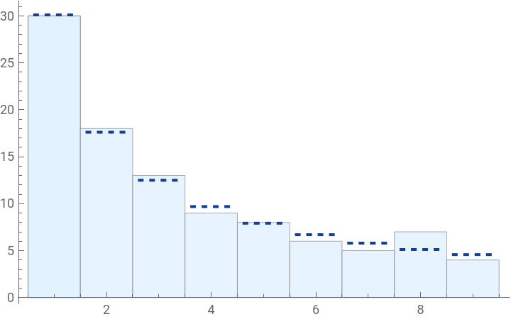


The first hundred digits of the Fibonacci sequence match the Benford distribution remarkably well. As is often the case with Benford sequences, there is a small discrepancy between the experimental distribution and theory. Like any data set that is expected to exemplify a specific distribution (e.g. data for normal distributions), analyzing more data points often leads to a closer match. This is the very concept we will use to measure convergence to Benford distribution.
3) Computational Framework
3) Computational Framework
3.1) Total Variation
3.1) Total Variation
Definition
Definition
Comparing convergence of first digit frequencies to the Benford distribution across different sequences necessitates the use of a formal metric. Throughout this paper we will use total variation as a means to measure the difference between the experimental first digit distribution of a sequence to the expected Benford distribution across any number of terms. Consider a sequence with N terms. Letting d ∈ { 1, 2, .... , 9 }, define as the observed relative frequency of leading digit d, and (d) as the Benford probability for digit d. So = (# of starting with d) / N and = (1 + ) . Total variation is defined as
N
{}
a
n
n=1
P(d)
Q
P(d)
a
n
Q(d)
log
10
1
d
1 2 9 ∑ d=1 |
Note that (P,Q) ∈ [0 , 1]. Intuitively, the closer the sets P and D are, the closer total variation will be to zero. Thus, if the experimental relative frequencies match the Benford distribution exactly, total variation will equal zero.
D
TV
Plotting Total Variation
Plotting Total Variation
As mentioned earlier, the number of terms N of a sequence you include in your analysis will affect the relative frequencies of the leading digits. This means depends on N.
Hence, total variation is a function of N. Let’s alter the notation to reflect this:
P(d)
Hence, total variation is a function of N. Let’s alter the notation to reflect this:
1 2 9 ∑ d=1 P N |
This naturally led to the decision to plot total variation for different sequences in order to observe their convergence behavior.
3.2) Constructing Reusable Functions
3.2) Constructing Reusable Functions
I needed my own library of functions to reuse for each sequence. It was important that they be versatile and efficient to handle large data sets (up to 100 000 terms). They are each designed to deal with an input that is a list of sequence terms, with no index numbers. There is also data stored about Benford’s function both to use in total variation calculations and to refer back to for comparison. Let’s start by simply generating a table of the Benford probabilities which will be repeatedly used throughout this computational study.
Make a table of expected Benford frequencies:
In[]:=
benfordProb=Table[{d,N[Log10[1+1/d],30]},{d,1,9}];benfordProb//TableForm
Out[]//TableForm=
1 | 0.301029995663981195213738894724 |
2 | 0.176091259055681242081289008531 |
3 | 0.124938736608299953132449886194 |
4 | 0.0969100130080564143587833158265 |
5 | 0.0791812460476248277225056927041 |
6 | 0.0669467896306131982034494606130 |
7 | 0.0579919469776867549290004255808 |
8 | 0.0511525224473812889488391223368 |
9 | 0.0457574905606751254099441934898 |
For each sequence I will need a function to extract the first digits of each term and turn it into a list. This will be accomplished using the built in function: IntegerDigits
firstDigits[data_List]:=IntegerDigits[data][[All,1]];
Count the leading digit occurrences for each digit and output an association:
In[]:=
digitCounts[dig_List]:=Counts[dig];
Construct a function that counts the leading digit numbers and computes empirical frequencies by dividing by n. This function calls firstDigits inside, so the parameter is just the sequence terms. Output is a list of ordered pairs.
In[]:=
freqsData[myData_List]:=Table[{d,Lookup[digitCounts[firstDigits[myData]],d,0]/Length[myData]},{d,1,9}];
Create a plot of Benford’s Law to use to compare empirical frequencies.
In[]:=
benfordPlot=PlotLog10[1+1/x],{x,1,9},;
Test plot comparison with the first 20 Fibonacci terms :
In[]:=
testSequence=Table[Fibonacci[n],{n,1,50}];testFreqs=freqsData[testSequence]
Out[]=
1,,2,,3,,4,,5,,6,,7,,8,,9,
8
25
9
50
3
25
2
25
2
25
3
50
3
50
3
50
1
25
In[]:=
In[]:=
testPlot=ListPlot[testFreqs];Labeled[Show[benfordPlot,testPlot],Text[Style["Note that Benford's Law is defined only for integers. \nRepresented as continuous for visualization.",Gray,12]],Bottom,Spacings->10]
When I first put this code together, I made functions individually to count the number of leading digits, then convert to frequency data and finally compute the total variation. This worked find for up to about ten thousand terms, but I quickly found that it was not efficient enough. So instead I combined them into the following function which is faster because it updates the digit counts incrementally as each new term is processed, rather than recomputing the frequencies from scratch for every value of N. As a result, each iteration performs only a constant amount of work, making the overall algorithm much more efficient for large sequences.
Consider the terms of the sequence one at a time, beginning with the first term, incrementing by step, and terminating with the full sequence. As a new term is processed, the counts of the leading digits are updated incrementally. At each sampling point, the digit frequencies are obtained by dividing these counts by the number of terms currently analyzed, and the resulting frequency distribution is used to compute the total variation.
Perform a simple test to demonstrate and confirm functionality:
In the above plot, we see total variation getting smaller as the number of terms analyzed increases. This is exactly what we expect in a sequence that is known to satisfy Benford’s Law.
But, should it actually trend towards zero?
But, should it actually trend towards zero?
Theorem 3.3 (Equivalence of Benford Behavior and Total Variation Convergence)
Theorem 3.3 (Equivalence of Benford Behavior and Total Variation Convergence)
Therefore,
Since all terms in the sum are non-negative,
According to the above result, for any sequence that is known to satisfy Benford’s Law we expect to see the total variation plot eventually approach zero. Conversely, we have also proved that if a total variation plot indeed converges to zero, that is equivalent to the sequence satisfying Benford’s Law.
4) Benford Sequences
4) Benford Sequences
4.1) Fibonacci Sequence
4.1) Fibonacci Sequence
As mentioned earlier, Fibonacci is possibly the single most famous example of a Benford sequence. We’ve now seen a sample total variation plot for the first thirty terms of the sequence.
As shown in Theorem 3.3, since Fibonacci is known to satisfy Benford’s Law, we should expect the total variation plot to eventually converge to zero.
As shown in Theorem 3.3, since Fibonacci is known to satisfy Benford’s Law, we should expect the total variation plot to eventually converge to zero.
The first thing we need is a way to generate the first n terms of the Fibonacci sequence into a list.
Example:
Now create data of the total variation using the benfordConvergence function we built earlier. Let’s start with 10,000 terms, beginning at 100 with a step of 10:
Several observations are immediate. First, as predicted the plot continues to decrease, however it is not monotone and includes an interesting spikey oscillation pattern. This means that for some reason the Fibonacci sequence has periods of roaming further from Benford’s distribution even though it eventually converges. Note that when I saw roaming further away the keyword is further because relatively speaking for this number of terms a total variation of 0.002 even is incredibly small.
Let’s observe the relative frequences on top of the Benford distribution. Since benfordConvergence handles the frequency calculations internally, we will have to reproduce it here:
The above plot indicates that a total variation of 0.002 is impossible to note visually. If we created a histogram of the leading digits in these 10 000 Fibonacci terms, it would not be distinguishable from perfect Benford distribution. However, Theorem 1.1 states that the total variation should converge to zero, and hence get even closer. Let’s push it further.
Create and plot data for the first 100 000 terms of Fibonacci:
Use FindFit function to fit values of a and b using the generated total variation data to our chosen model:
Create a function to store our fit values and plot it:
Note our fit function is undefined at zero, so we start a bit after:
Theorem 4.2 (Benford Property of Power Sequences)
Theorem 4.2 (Benford Property of Power Sequences)
This theorem is a standard result .
The length of this interval is
Note. The proof relies on Weyl’s Equidistribution Theorem, whose proof is beyond the scope of this essay. Although this study generally favors self contained arguments, Weyl’s theorem is taken as a standard number theory result.
Create a table of n terms of our sequence. This time we will have to define the sequence itself first.
Now let’s save the total variation data using benfordConvergence function again and plot it:
Traces of the interesting oscillation observed in the Fibonacci total variation decay plot are observable in the powers of two sequence as well. We can also see overall the same shape of convergence. Let’s try the same fit function.
Plot the fit function and display with the total variation data:
This fit seems to slightly overestimate the data at points, but overall is decent.
Sequence Definition:
Generate total variation data and plot:
Find the fit:
The oscillations in the convergence graph of the power of three sequence seem sharper with a shorter period than the previous two sequences. The recurring spikes are intriguing and merit further investigation; their in depth analysis lies beyond the scope of the present study. Part of what appears most interesting is the fact that the observed structure does not appear to arise from interactions between consecutive terms, but rather emerges collectively from the full set of evaluated points, with the visual pattern becoming apparent when the data are viewed as a whole.
Sequence Definition:
Generate total variation data and plot:
Find the fit:
Note. Values on the left of the graph have been cut off by limiting the range. Shortening the range allows the pattern in the plot to be seen more clearly.
It was at this point in the study that the terms were growing too large and the computations too cumbersome for the benfordConvergence function.
The answer to reducing computing time was in the fact that with each term benfordConvergence was computing more than necessary because we did not need the full term, only the first digit.
The answer to reducing computing time was in the fact that with each term benfordConvergence was computing more than necessary because we did not need the full term, only the first digit.
Construct the first digit by raising ten to the fractional part of each logarithm and apply floor:
Let’s double check that power5Digits is doing what we expect:
Since the benfordConvergence function computes leading digits inside, it is expecting a list of sequence terms as it. Since we managed to jump straight to the first digits, we should write a new version of the function that skips over that step.
Remove the local variable from benfordConvergence and rename (so the old one is still usable):
Generate total variation data and plot:
Find the fit:
The same method we used to streamline the base 5 power sequence we can use for the base 6 sequence.
Update the inside of the logarithm for base 6 power sequence:
Compute the total variation data for powers of six remembering to use benfordConvergenceFromDigits:
Find the fit:
Onto base 7:
Update the inside of the logarithm for base 7 power sequence:
Compute the total variation data for powers of seven remembering to use benfordConvergenceFromDigits:
4.3) Shifted Sequences
4.3) Shifted Sequences
Shifted Fibonacci
Shifted Fibonacci
As we’ve established multiple times, Fibonacci converges nicely to the Benford distribution.
Although it is well known that additive shifts generally do not preserve Benford distributions for finite data sets, this does not necessarily determine the asymptotic behavior of an infinite sequence.
So, in the experimental study mindset, I decided to just try it and see.
Although it is well known that additive shifts generally do not preserve Benford distributions for finite data sets, this does not necessarily determine the asymptotic behavior of an infinite sequence.
So, in the experimental study mindset, I decided to just try it and see.
Let’s begin by adding 1111 to every term.
Construct the Sequence:
Total Variation Data:
The following code is the same process used for all previous sequences. Iconized for visual clarity.
Clearly this new shifted Fibonacci sequence also satisfies Benford’s Law eventually.
Let’s Compare this fit to the original Fibonacci fit:
As we can see above the shift caused the sequence to converge slower, but only marginally. This observation suggests the asymptotic behavior of unbounded sequences may differ from the finite data setting.
I played around with a few more sequences, shifting them around by various constants. All yielded the same result: shifting by a constant changed the rate of convergence, and total variation in lower numbers of terms, but ultimately did not change asymptotic behavior. So began a period of internet sleuthing. I sniffed around all sorts of literature on Benford’s Law and the theories behind it.
I played around with a few more sequences, shifting them around by various constants. All yielded the same result: shifting by a constant changed the rate of convergence, and total variation in lower numbers of terms, but ultimately did not change asymptotic behavior. So began a period of internet sleuthing. I sniffed around all sorts of literature on Benford’s Law and the theories behind it.
In the end the proof is rather simple, and relies on a standard result from uniform distribution theory.
Lemma: (Standard result from uniform distribution theory) See: Chapter 1, Theorem 1.2, Uniform Distribution of Sequences, L. Kuipers and H. Niederreiter.
Theorem 4.3 (Asymptotic Preservation of Benford Behavior)
Theorem 4.3 (Asymptotic Preservation of Benford Behavior)
Define
Then
4.4) n! and Similarly Growing Sequences
4.4) n! and Similarly Growing Sequences
4.5 a) n!
4.5 a) n!
Factorials are everywhere in mathematics. It would be wrong to perform a study such as this without analyzing the factorial sequence for Benford behavior.
Due to the extremely fast growth rate, analyzing the factorial sequence became extremely computationally heavy extremely fast. As such I have decided to cap the following total variation plot at 50 000 terms instead of 100 000.
The factorial sequence was the first sequence I found exhibiting this new total variation plot shape. Noting the scale of the y-axis, we can see that overall it decays less swiftly than the exponentially growing functions (the Fibonacci sequence also has an exponential growth rate).
The other sequence I came across that also grows faster than exponential, is a modified version of the Fibonacci sequence, where you multiple the second term by n.
4.5) Comparison of Convergence Rates
4.5) Comparison of Convergence Rates
Now that we have examined different total variation plots many with a power law decay pattern, it seems a worthwhile pursuit to compare their best fits.
The total range for the fit variable b for this sequence set is [ 0.8513 - 0.974 ]. Although analyzing more sequences would likely extend this range, it is remarkably close for such different sequences including both Fibonacci +1111 and integer power sequences. Note that the Fibonacci sequence grows at a rate roughly equivalent to the power sequence base Golden Ration (φ = ~1.618 ) which could be a factor in the similar convergence rates.
5)Non-Benford Sequences
5)Non-Benford Sequences
Two classes of sequences were of particular interest in this investigation: the prime numbers and nestedly recursive sequences. Although neither class was found to converge to Benford’s Law, both exhibited remarkably consistent and reproducible patterns in their total variation distance from the Benford distribution. These patterns persisted across increasingly large samples, suggesting that even non-Benford sequences may possess characteristic convergence signatures. Understanding these signatures may provide additional insight into the relationship between sequence growth and leading-digit behavior.
5.1) The Sequence of Primes
5.1) The Sequence of Primes
A popular example of a sequence that does not satisfy Benford’s Law, the sequence of primes is a perfect place to examine patterns of first digit distribution in non-Benford sequences, with the purpose of providing material for later comparison.
5.2) Nestedly Recursive Functions
5.2) Nestedly Recursive Functions
Nestedly Recursive Functions are recursive functions that contain a function call within a function call. Of particular Interest to Stephen Wolfram, (See: Nestedly Recursive Functions) “NRFs” are a classic and fascinating example of ruliology. Most often being positive integer sequences it seemed reasonable that some or most would exhibit Benford Behavior. I investigated a wide variety of NRFs including many of the classic examples.
Memoization and initial conditions are required to define NRFs in WL:
Q(n) = Q( n - Q( n - 1)) + Q( n - Q(n - 2)) - Hofstadter’s Q Sequence
Q(n) = Q( n - Q( n - 1)) + Q( n - Q(n - 2)) - Hofstadter’s Q Sequence
(All of the NRFs will use the same initial terms as the Fibonacci sequence unless specified otherwise.)
This total variation plot showcases one small distinction from the others: the rounded tops at local maximums.
H(n) = n - H( H( H( n - 1))) - Hofstadter’s H Sequence
H(n) = n - H( H( H( n - 1))) - Hofstadter’s H Sequence
For Hofstadter’s H sequence, H[0] = 0. Often Initial conditions must be altered to avoid recursion errors. Additionally, it is very hard to test a large variety of initial conditions and their impact on Benford behavior due to their tendency towards recursion error.
It was around this point that I began to suspect the role in the slow linear like growth of NRFs as a factor in their leading digit distribution :
After much scouring of the literature on nestedly recursive functions I was unable to find one that exhibited a faster growth rate, for the same limiting factor that I ran into trying to test different initial terms. The sensitivity of NRFs to recursion error is a result of the very thing that makes them interesting: nested recursion. Even taking measures such as assigning any negative n value to the output of 1, was not enough to produce any faster growing NRFs.
c(n) = c( n - c( n - 1)) + c( n - 1 - c( n - 2)) - Meta-Fibonacci Sequence (Conelly-Newman Type)
c(n) = c( n - c( n - 1)) + c( n - 1 - c( n - 2)) - Meta-Fibonacci Sequence (Conelly-Newman Type)
A(n) = A( A( n - 1)) + A( n - A( n - 1)) - Hofstadter-Conway $10,000 Sequence
A(n) = A( A( n - 1)) + A( n - A( n - 1)) - Hofstadter-Conway $10,000 Sequence
Effect of Growth Rate on Benford Behavior in NRFs:
Effect of Growth Rate on Benford Behavior in NRFs:
One hypothesis for the sawtooth pattern observed in nestedly recursive sequences is their approximately linear growth. As the order of magnitude increases, the sequence spends progressively longer intervals among terms beginning with the same leading digit before transitioning to the next leading digit. This prolonged accumulation and subsequent depletion of individual leading digits may alternately increase and decrease the total variation distance from the Benford distribution, producing the observed sawtooth pattern. Further investigation would be required to determine whether this behavior is an inherent consequence of approximately linear growth or a feature specific to the nestedly recursive sequences examined.
Concluding Remarks and Future Direction
Concluding Remarks and Future Direction
Acknowledgements
Acknowledgements
I would like to express my gratitude to Jesús Montesinos for serving as my mentor throughout this project. His guidance and thoughtful feedback were invaluable to the development of this work. I am also grateful to Stephen Wolfram for proposing this research topic during the Wolfram Summer Research Institute and for providing the opportunity to explore it. Additionally, I would like to thank Utkarsh Bajaj for his support as a teaching assistant and for his assistance throughout the project.
References
References
1
.Wang, L. & Ma, B.Q. (2024), “A Concise Proof of Benford’s Law”, Fundamental Research. https://www.sciencedirect.com/science/article/pii/S2667325823000043
2
.Murtagh, J. (2023), “What is Benford’s Law? Why This Unexpected Pattern of Numbers Is Everywhere”, Scientific American. https://www.scientificamerican.com/article/what-is-benfords-law-why-this-unexpected-pattern-of-numbers-is-everywhere/
3
.Berger, A. & Hill, T.P. (2017), “What is Benford’s Law”, Notices of The American Mathematical Society. https://www.ams.org/journals/notices/201702/rnoti-p132.pdf
4
.Miller, S.J. & Nigrini, M.J. (2007), “The Modulo 1 Central Limit Theorem and Benford’s Law For Products”, International Journal of Algebra. https://web.williams.edu/Mathematics/sjmiller/public_html/math/papers/Mod1CLT_BenfProd10.pdf
5
.Wolfram, S. (2024), “Nestedly Recursive Functions”, Stephen Wolfram Writings. https://writings.stephenwolfram.com/2024/09/nestedly-recursive-functions/
6
.Yifrach, Y. (2023), “A Note on Weyl’s Equidistribution Theorem”, ArXiv Preprint. https://arxiv.org/abs/2201.07138
7
.Kuipers, L. & Niederreiter, H. (1974), Uniform Distribution of Sequences. Wiley-Intersciences Publishing. https://web.maths.unsw.edu.au/~josefdick/preprints/KuipersNied_book.pdf
8
.Berger, A. & Hill, T. (2015), An Introduction to Benford’s Law, Princeton University Press. https://books.google.com/books?id=BfRnBgAAQBAJ&pg=PA1&source=gbs_toc_r&cad=2#v=onepage&q&f=false
9
.Hyman, M. (2026), “Why Eight Percent of Benford Sequences Never Converge”, ArXiv Preprint. https://arxiv.org/pdf/2603.18243
AI Disclosure
AI Disclosure
The following generative AI tools were used in this project: [ChatGPT- 5.5]. It was used for minor debugging and theoretical consultation. All final code, theorems, analysis and written content was produced by the author or otherwise appropriately cited.
CITE THIS NOTEBOOK
CITE THIS NOTEBOOK
A Computational Study of Benford's Law in Integer Sequences
by Sonia Wolgamot
Wolfram Community, STAFF PICKS, July 16, 2026
https://community.wolfram.com/groups/-/m/t/3762954
by Sonia Wolgamot
Wolfram Community, STAFF PICKS, July 16, 2026
https://community.wolfram.com/groups/-/m/t/3762954