ORIGINAL ARTICLE: George D. Xavier, M-CHIPR: A Mathematica program for constructing multi-state coupled adiabatic potential energy functions in triatomic molecule using many body partitioning approach, Comput. Phys. Comm. 278 (2022) 108419. DOI: https://doi.org/10.1016/j.cpc.2022.108419
Article Abstract: The permutationally invariant combined hyperbolic inverse power representation (CHIPR) polynomial expansion in terms of hyperbolic secant basis proves to be an efficient model in describing the multi state coupled potential energy surface (MSCPES) and this fact was tested on the triatomic ion and its diatomic sub units upon dissociation with an unmatchable accuracy of fitting in comparison with the previous works (below 1 in the case of diatomic function and below 300 in the case of triatomic function). In general, this model is capable of modeling (,etc.) and ABC (OCS, etc.) triatomic system in addition to the B system. This paper presents a Mathematica notebook (M-CHIPR.nb file) to perform the fitting of di and triatomic potentials in a user friendly manner with proper explanations written along side wherever required in the .nb file supplied. The advantage of this code is that the computing clusters are not required to use it and can be run in normal pc with good processor and memory, apart from its numerical accuracy and the system independent consistency over the similar programs written in other languages.
O
2
+
H
-1
cm
-1
cm
A
3
H
3
O
3
+
HCO
A
2
()
O
2
+
H
Introduction
Introduction
This note book contains Mathematica code to fit the diatomic and triatomic ab initio data and seam trajectory using the eigen value expression of 2 by 2 diabatic matrix
M-CHIPR is a Mathematica note book that can be downloaded and used for the above mentioned purpose by any one. The result from using this code appeared in few articles in the past. The user can consult them if they so wish.
The following sections describe the details about the model function and Mathematica command and how to use the code with proper syntax. The result is presented in the form of 2d and 3d plot. Comprehensive documentation and to run in Parallel can be found from Mathematica’s Documentation Center.
Diatomic script and its Application
Diatomic script and its Application
User can write their directory path where the file containing the fitting data lies. Example:/Users/a/b/c
SetDirectory["write users directory"];
Importing the data file named “OH+.dat” here with Import command and saved in another variable “dataohp” and the points not required can be deleted using Delete command, consult online manual
dataohp=Delete[Import["OH+.dat"],{{1},{2},{3},{4}}]
x is the linear combination mentioned in the manuscript and the number of terms can be altered to improve the fitting quality
x=Sechr1-+Sechr1-+Sechr1-+Sechr1-;
a
1
Tanhr1-
β
1
ζ
1
0
()
R
oh
0
()
R
oh
μ
1
ζ
1
0
()
R
oh
a
2
Tanhr1-
β
1
ζ
1
1
()
R
oh
1
()
R
oh
μ
2
ζ
1
1
()
R
oh
a
3
Tanhr1-
β
1
ζ
1
2
()
R
oh
2
()
R
oh
μ
3
ζ
1
2
()
R
oh
a
4
Tanhr1-
β
1
ζ
1
3
()
R
oh
3
()
R
oh
μ
4
ζ
1
3
()
R
oh
model is polynomial of degree 7(can be of any degree)in x basis defined in the previous line and saved in the variable anamod1. polynomial degree can be altered to improve the fit
anamod1=Sum,{i,7};
8
ω
r1
A
i
i
x
The line Mathematica does the fitting with Nonlinearmodelfit command on the data stored in datohp using the model anamod1 to find the unknown coefficients with the running variable named r1, the value 1.86 is the starting value given to
R
oh
fitoh=NonlinearModelFit[dataohp,{anamod1},{{,(*1.97*)1.86},{ω},,,,,,,,,,,,,,,,,},r1,MaxIterations32000];
R
oh
β
1
a
1
a
2
a
3
a
4
A
1
A
2
A
3
A
4
A
5
A
6
A
7
ζ
1
μ
1
μ
2
μ
3
μ
4
The optimized coefficients after the fitting run
fitoh["BestFitParameters"]
calculate root mean square error
Print"RMSD=",RootMeanSquare[Table[dataohp[[i]][[2]]-fitoh[dataohp[[i]][[1]]],{i,Length[dataohp]}]]219474.63,""
-1
cm
The user can adapt the following script to make their plot which will look nearly the same after making necessary changes to the script and also consulting mathematical manual regarding how to plot
Show[Plot[{fitoh[r],fito2p[r],fito2[r]},{r,0,50},PlotRange{{1.2,8},{-0.26,0.05}},FrameTicks{{2,4,6,8},{-0.25,-0.20,-0.15,-0.10,-0.05,0,0.05}},Epilog{Text[Style["",FontSize14],{6,0.1}]},Axes{False,True},FrameStyleDirective[16],LabelStyle{FontSize16},FrameLabel{"bond distance/bohr","energy/hartree"},Frame->True,PlotLegendsPlaced[{Style[" fit",White,14],Style[" fit",White,14],Style[" fit",White,14]},{Scaled[{0,0.5}],{-4.5,0.5}}],PlotTheme"Marketing"(*,GridLinesNone*)],ListPlot[{dataohp,datao2p,datao2},PlotLegendsPlaced[{Style["data",White,14],Style["data",White,14],Style["data",White,14]},{Scaled[{0,0.5}],{-3.95,1.5}}],PlotTheme"Marketing"],ImageSizeLarge]
+
O
2
+
OH
+
O
2
O
2
+
OH
+
O
2
O
2
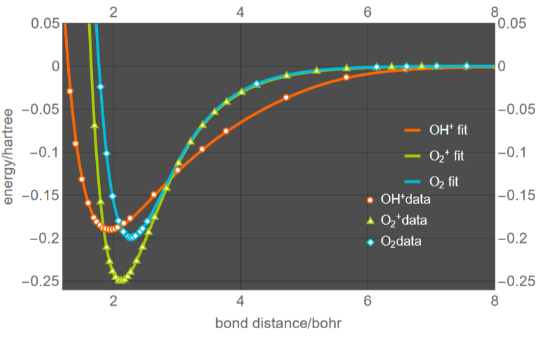
This plot is obtained by running the above script and rmsd obtained is below and the length of the contracted basis is not same for all diatomic species. For OH+, there are 4 terms and polynomial of degree 7 and for other two species, there are six terms with polynomial of degree 10. The user can adapt the above script for fitting the molecular data of their choice
1
-1
cm
Triatomic script and its Application
Triatomic script and its Application
Analytical model to fit the data of three body potential given in this script.
,, are the linear combination for A2B system, each one with five terms, but it can be changed to any number. Duration of fitting depends upon this number of terms, more the terms more the quality and heavier the computation. A minimum of 3 term is required to obtain meaningful fit. For other two types of molecular system, to write the expression for ,, please look at the manuscript. The expansion of polynomial is written up to the degree of 15, each degree with the correct number of monomial and their associated coefficients applicable to A2B system. For each degree, list of monomial are closed in parenthesis indicating the degree in pink. There is no need for user to use full expansion to fit initially. They can start with smaller expansion first and if not satisfied with the result, big expansion may be considered, sometimes overriding limit set in the code 15 to 16,17 etc by extending the expansion. Lastly, Mathematica key word to perform nonlinear fit is given and saved the arbitrary function called “fit” which is again called in the sequence fit[u,v,w] with replacement of variable, r1--->u,r2---->v,r3----->w. For example, fit[2,3,4] gives the result.
y
1
y
2
y
3
y
1
y
2
y
3
y
1
Tanhu-
β
1
ζ
1
0
()
R
ref1
0
()
R
ref1
γ
1
ζ
1
0
()
R
ref1
Tanhu-
β
1
ζ
1
1
()
R
ref1
1
()
R
ref1
γ
2
ζ
1
1
()
R
ref1
Tanhu-
β
1
ζ
1
2
()
R
ref1
2
()
R
ref1
γ
3
ζ
1
2
()
R
ref1
Tanhu-
β
1
ζ
1
3
()
R
ref1
3
()
R
ref1
γ
4
ζ
1
3
()
R
ref1
Tanhu-
β
1
ζ
1
4
()
R
ref1
4
()
R
ref1
γ
17
ζ
1
4
()
R
ref1
y
2
Tanhv-
β
2
ζ
2
0
()
R
ref2
0
()
R
ref2
γ
5
ζ
2
0
()
R
ref2
Tanhv-
β
2
ζ
2
1
()
R
ref2
1
()
R
ref2
γ
6
ζ
2
1
()
R
ref2
Tanhv-
β
2
ζ
2
2
()
R
ref2
2
()
R
ref2
γ
7
ζ
2
2
()
R
ref2
Tanhv-
β
2
ζ
2
3
()
R
ref2
3
()
R
ref2
γ
8
ζ
2
3
()
R
ref2
Tanhv-
β
2
ζ
2
4
()
R
ref2
4
()
R
ref2
γ
9
ζ
2
4
()
R
ref2
y
3
Tanhw-
β
2
ζ
2
0
()
R
ref2
0
()
R
ref2
γ
5
ζ
2
0
()
R
ref2
Tanhw-
β
2
ζ
2
1
()
R
ref2
1
()
R
ref2
γ
6
ζ
2
1
()
R
ref2
Tanhw-
β
2
ζ
2
2
()
R
ref2
2
()
R
ref2
γ
7
ζ
2
2
()
R
ref2
Tanhw-
β
2
ζ
2
3
()
R
ref2
3
()
R
ref2
γ
8
ζ
2
3
()
R
ref2
Tanhw-
β
2
ζ
2
4
()
R
ref2
4
()
R
ref2
γ
9
ζ
2
4
()
R
ref2
1
8
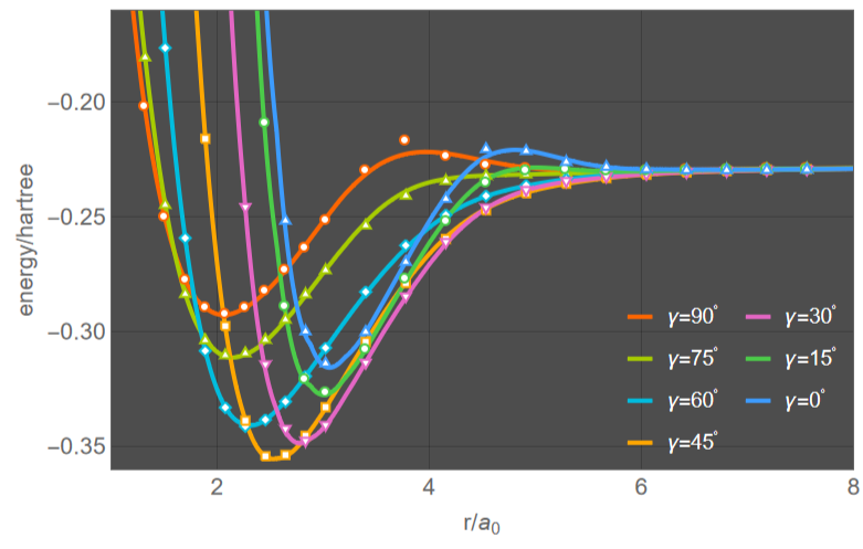
A 2d cut of model function for various Jacobi angle as a function of bond distance
O
2
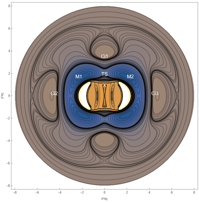
A relaxed Plot of mode function by relaxing as a function of distance between cm and expressed in Cartesian coordinates
O
2
+
H
Two state cusp fitting
Two state cusp fitting
Hyperspherical surface of two states showing cusp and respective geometires
Diatomic Curves (Tested Examples)
Diatomic Curves (Tested Examples)
Calculation of Three Body Potentials in Valence Coordinates/Conversion from Jacobi to Valence Coordinates
Calculation of Three Body Potentials in Valence Coordinates/Conversion from Jacobi to Valence Coordinates
CITE THIS NOTEBOOK
CITE THIS NOTEBOOK