This Wolfram Mathematica notebook is a template that can be used for most homework problems a university student might see in the first few chapters of a differential equations textbook. This handful of simple plots and equations also makes discrete numerical (T)ables and Lists. Just by changing a few entries the picture below can be flipped around, stretched and “scaled”. The entire worksheet can then be re calculated to show the numerical Matrix that matches the curves in the graph. Ultimately, the picture below will become a mathematical motion picture. The student must demonstrate some ability to use the Manipulate and other similar commands to Show the Calculus in action (a daunting excercise in computer syntax).The student must lecture the mathematics and do the work on the chalkboard using the computer movie as a tool only for the minimum grade. Using any other popular computer algebra system (MatLab, Mathcad) or any of the multitudes of engineering website/platforms for mathematics and science, to accomplish pretty much the same thing, even when using the different software, for the first time is a pre requisite. Even the graphing calculator many high school students still use and most professors learned with, can “show” differential calculus not in action but holding still in black and grey screen and a tiny AspetcRatio waiting for the computer age. Ultimately, when finished, the student must use a cell phone and speak, without doing any math (this is a requirement) the same mathematical movie (with color) into existence and show it to your friends . . . on your phone. Wolfram Mathematica / Wolfram Alpha and most other high order “artificial intelligence” softwares can do this with ease.
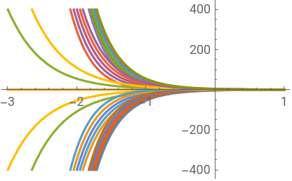
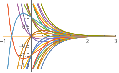
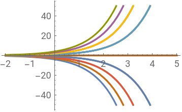
Using small numbers like two and three, paying attention to the negative exponent , we assemble the simplest differential equation with minus two and three showing up as factors in the exponents. Try plus two and plus three, or minus three and plus two, and watch the picture flip back and forth. Write a mathematical novel about what you just did on the computer and how much time it would have taken to calculate all that on paper.
y[x]:=a*Exp[-2x]+b*Exp[-3x]
Plot[Evaluate[Table[y[x],{a,-2,2},{b,-2,2}]],{x,-3,1}]
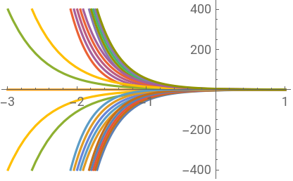
The equation we choose is minus two and minus three for the factor we will multiply the variable x in the exponent of eulers number e. Which is why we choose the following homework problem to practice.Solve the differential equation x + 5 + 6y = 0
^2
x
x
Clear[y]
solution=DSolveValue[{y''[x]+5y'[x]+6y[x]0},y[x],x]
-3x
-2x
solutiontable=Table[solution/.{C[1]i,C[2]j},{i,-2,2},{j,-2,2}]
{{-2-2,-2-,-2,-2+,-2+2},{--2,--,-,-+,-+2},{-2,-,0,,2},{-2,-,,+,+2},{2-2,2-,2,2+,2+2}}
-3x
-2x
-3x
-2x
-3x
-3x
-2x
-3x
-2x
-3x
-2x
-3x
-2x
-3x
-3x
-2x
-3x
-2x
-2x
-2x
-2x
-2x
-3x
-2x
-3x
-2x
-3x
-3x
-2x
-3x
-2x
-3x
-2x
-3x
-2x
-3x
-3x
-2x
-3x
-2x
TableForm[solutiontable]
-2 -3x -2x | -2 -3x -2x | -2 -3x | -2 -3x -2x | -2 -3x -2x |
- -3x -2x | - -3x -2x | - -3x | - -3x -2x | - -3x -2x |
-2 -2x | - -2x | 0 | -2x | 2 -2x |
-3x -2x | -3x -2x | -3x | -3x -2x | -3x -2x |
2 -3x -2x | 2 -3x -2x | 2 -3x | 2 -3x -2x | 2 -3x -2x |
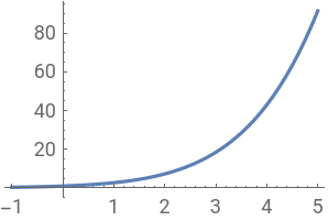
Normal[Series[Exp[x],{x,0,5}]]
1+x++++
2
x
2
3
x
6
4
x
24
5
x
120
Plot1+x++++,{x,-1.,5}
2
x
2
3
x
6
4
x
24
5
x
120
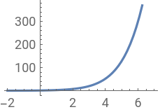
Plot1+x++++++,{x,-2,7}
2
x
2
3
x
6
4
x
24
5
x
120
6
x
720
7
x
5040
Clear[y]
solution=DSolveValue[{y''[x]+y'[x]+y[x]0},y[x],x]
-x/2
3
x2
-x/2
3
x2
solutiontable=Table[solution/.{c[1]i,c[2]j},{i,-2,2},{j,-2,2}]
{{C[1]+C[2],C[1]+C[2],C[1]+C[2],C[1]+C[2],C[1]+C[2]},{C[1]+C[2],C[1]+C[2],C[1]+C[2],C[1]+C[2],C[1]+C[2]},{C[1]+C[2],C[1]+C[2],C[1]+C[2],C[1]+C[2],C[1]+C[2]},{C[1]+C[2],C[1]+C[2],C[1]+C[2],C[1]+C[2],C[1]+C[2]},{C[1]+C[2],C[1]+C[2],C[1]+C[2],C[1]+C[2],C[1]+C[2]}}
-3x
-2x
-3x
-2x
-3x
-2x
-3x
-2x
-3x
-2x
-3x
-2x
-3x
-2x
-3x
-2x
-3x
-2x
-3x
-2x
-3x
-2x
-3x
-2x
-3x
-2x
-3x
-2x
-3x
-2x
-3x
-2x
-3x
-2x
-3x
-2x
-3x
-2x
-3x
-2x
-3x
-2x
-3x
-2x
-3x
-2x
-3x
-2x
-3x
-2x