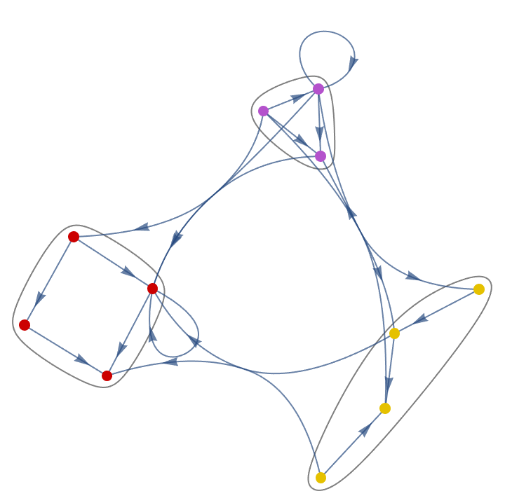
Simulating quantum Hamiltonians is both a flagship application of future quantum computers and also of theoretical interest. Here, we demonstrate how graph neural networks can be used to learn weights in target Hamiltonians representing the quantum Ising chain. We demonstrate how the weights in a maximally connected graph describing next-to-nearest interactions are turned off when learning the target Hamiltonian and also consider time evolutions to study the propagating errors.
Applying Graph Neural Networks to Quantum Hamiltonians
Applying Graph Neural Networks to Quantum Hamiltonians
Certain many-body Hamiltonians admit a graph structure with weights either in the form of interaction strengths between atoms in a molecule or the coefficients of initial quantum state itself (see this paper). Using GNNs one can learn the weights associated to such Hamiltonians with neural networks and then simulate the evolution in a straightforward manner.
Here, the goal is to use GNNs to learn the weights associated to the ground state of a well-studied and simple quantum model, the quantum transverse field Ising chain. For our purposes, we are going to learn the ground state of the following target Hamiltonian for a -qubit system
n
In[]:=
H
Ising
∑
〈i,j〉
ω
ij
Z
i
Z
j
∑
i
X
i
where are the Pauli spin matrices which are meant to represent a qubit at the node site with spin pointing along the respective bases and is meant to represent the nearest neighbor interactions. Here is the set of interaction weights. Let’s discuss the graph structure of this model briefly. For a more in-depth look, including phase transitions, magnetization, and entanglement structure, see an earlier computational essay and here.
X,Z
i,j
〈i,j〉
ω
ij
Boundary Conditions
Boundary Conditions
First, let’s consider the boundary conditions. The -qubit system can either have periodic boundary conditions corresponding to a closed graph or free boundary conditions corresponding to an open graph. We can design an -qubit system with either boundary condition in the following way. Let the list of pair interactions in the target Hamiltonian be given by
n
n
In[]:=
(*ListofpairinteractionsinthetargetHamiltonian*)pbcs=True;pairlist[n_]:=SortBy[Sort/@If[pbcs,Join[Partition[Range[n],2,1],{{n,1}}],Partition[Range[n],2,1]],First];edgelist[n_]:=EdgeList[pairlist[n]]
where we have created a boolean variable pbcs (for periodic boundary conditions) initially set to be True. The pair interactions define the edges and the links in an -qubit system simultaneously. To understand how this works consider the following
n
In[]:=
(*Variousn-qubitconfigurations*)nqbmax=5;TableFormpbcs=False;Table[Show[Graph[pairlist[i],PlotTheme->"Web"],ImageSize->Tiny],{i,2,nqbmax}],Table[pairlist[i],{i,2,nqbmax}], pbcs=True;Table[Show[Graph[pairlist[i],PlotTheme->"Web"],ImageSize->Tiny],{i,2,nqbmax}],Table[pairlist[i],{i,2,nqbmax}], TableHeadings->{{"System w/ Free Edges","Edges & Links","System w/ Periodic Links","Edges & Links"},Table[i"-qubits",{i,2,nqbmax}]}
Out[]//TableForm=
2-qubits | 3-qubits | 4-qubits | 5-qubits | |||||||||||||||||||||||||||||
System w/ Free Edges | ||||||||||||||||||||||||||||||||
Edges & Links |
|
|
|
| ||||||||||||||||||||||||||||
System w/ Periodic Links | ||||||||||||||||||||||||||||||||
Edges & Links |
|
|
|
|





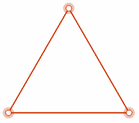
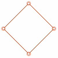
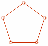
Above we have configurations where the qubits, sitting at the links, are connected to their nearest neighbors. When the qubits at the ends of the chains are allowed to form an additional edge, we have a closed graph (corresponding to periodic boundary conditions). Henceforth, we will set and work with closed graphs.
pbcs=True
Target Hamiltonians & Ground States
Target Hamiltonians & Ground States
We can easily construct the target Ising Hamiltonian for an -qubit system and find its ground state using the Wolfram Quantum Framework.
n
In[]:=
PacletInstall[CloudObject["https://wolfr.am/DevWQCF"],ForceVersionInstall->True]<<Wolfram`QuantumFramework`
Out[]=
PacletObject

In[]:=
targetweights[nq_]:=Table,{i,nq};IsingHamiltonian[weights_,edges_,n_]:=weights.(QuantumOperator["Z",#]&/@edges)+Total@Table[QuantumOperator["X",{i}],{i,n}];
RandomInteger[{1,nq}]
nq
Henceforth, we will focus on a four-qubit Ising chain with periodic boundary conditions with only nearest-neighbor interactions turned on
In[]:=
nqubits=4;targetweightsnq=targetweights[nqubits];targetHnq=IsingHamiltonian[targetweightsnq,pairlist[nqubits],nqubits];
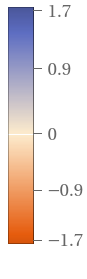
For this chain, we have the following target graph with random weights and the corresponding target Hamiltonian that we would like the GNN to learn
In[]:=
IsingChainEdges=edgelist[nqubits];(*TargetEdges*)presets={VertexLabelStyle->Directive[FontSize->14,FontWeight->Bold],VertexSize->Small,PlotTheme->"Web",EdgeStyle->Thick};EdgeLabelCoords={{1,0},{1,1},{0,0},{0,1}};targetgraph=GraphIsingChainEdges,presets,VertexLabels->Table[i->Placed[,Center],{i,Length[IsingChainEdges]}],EdgeLabels->TableIsingChainEdges[[i]]->PlacedStyle,FontSize->16,FontWeight->Bold,{1/2,EdgeLabelCoords[[i]]},{i,Length[IsingChainEdges]};tHnq=Normal[targetHnq["Matrix"]];Show[#,ImageSize->Small]&/@{targetgraph,MatrixPlot[tHnq,PlotTheme->"Scientific",PlotLegends->Automatic]}
ℋ
i
HoldForm[Ω]
IsingChainEdges[[i]]
Out[]=
,
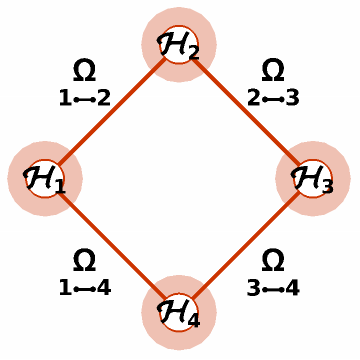
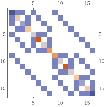
where the target weights are given by
In[]:=
Table=targetweightsnq[[i]],{i,Length[IsingChainEdges]}
Ω
IsingChainEdges[[i]]
Out[]=
,,,
1
2
3
4
1
4
1
4
In order to find the ground state of the system, we simply need to find the most negative eigenvalue of the Hamiltonian, i.e., the ground state energy
In[]:=
TableForm[{eigenval,eigenvecs}=Eigensystem[N[tHnq],2],TableHeadings->{None,{"",""}}]
E
1
E
2
Out[]//TableForm=
E 1 | E 2 | ||||||||||||||||||||||||||||||||
4.24095 | -4.24095 | ||||||||||||||||||||||||||||||||
|
|
We will evolve the above state once the GNN has learned the target Hamiltonian.
The 4-Qubit Initial GNN Ansatz
The 4-Qubit Initial GNN Ansatz
The aim is to learn these weights given an initial Hamiltonian
where the initial weights are given by
Learning the Target Hamiltonian
Learning the Target Hamiltonian
Since the initial weights and the target weights are of different dimension, let’s construct a final target weight vector of the same dimension.
Then fill in the entries of the finaltargetweights with the target weights, leaving the non-nearest neighbor interactions as zero.
Now, we have the data that we need to use to train the neural network
NetTrain trains the specified neural NetChain by giving data as an input and minimizing the discrepancy between the output and the actual output of the net. The NetChain I used is a 5-layer network with a LinearLayer of 150 nodes, a Tanh function, LinearLayer of 150 node, a LogisticSigmoid layer, and a single LinearLayer output layer. Using less/more functions will under/overtrain the neural network. In our case, we would like the GNN to model the data effectively so I used more functions. The results are below
Above is the trained neural network where the data points are the target weights and the curve is the networks best fit to the data. We see that if we feed in the initial weights, the trained network provides trained weights
and the difference between the trained weights and the target weights is
Hence, we have the following results from applying the GNN
where the errors between the target and trained Hamiltonian are sufficiently small. By training the neural network with different functions, longer times, more layers, or with larger batch sizes, it is possible to further minimize the difference. As another error estimation parameter, the difference in the expectation value of both Hamiltonians acting on the ground state, i.e.,
Evolving Quantum States and Error Characterization
Evolving Quantum States and Error Characterization
Now, that we have learned the target Hamiltonian to a sufficient degree, we can utilize the trained final Hamiltonian to study quantum dynamics. Let’s study the time evolution of the ground state with the trained and the target Hamiltonian and characterize the resulting error between the target and trained final Hamiltonian when performing a measurement.
We can define the time evolution operator as
We can define the time evolution operator as
and consider the time domain:
Errors in Evolved Ground States
Errors in Evolved Ground States
We construct the following error measure which characterizes the difference between evolved ground states with the corresponding operators
Although the error in the evolved ground states grows in time, the GNN is sufficiently well trained and the corresponding GNN energy eigenvalues predictions remain close to the target eigenvalues.
Conclusions
Conclusions
Given information about the target graph weights in a particular Hamiltonian, it is possible to learn such weights with graph neural networks and simulate the evolution of the Hamiltonian to characterize the error in the corresponding ground state.
Clearly, this is an idealized example and in the future, it should be possible to directly learn the target graph weights, characterize errors, and implement this process directly on a quantum circuit utilizing Quantum Graph Recurrent Neural Networks (see this paper).
Clearly, this is an idealized example and in the future, it should be possible to directly learn the target graph weights, characterize errors, and implement this process directly on a quantum circuit utilizing Quantum Graph Recurrent Neural Networks (see this paper).
Acknowledgements
Acknowledgements
I appreciate the Wolfram Quantum Framework team for feedback, in particular Nik Murzin and Mads Bahrami, along with William Munizzi who introduced/discussed various graph aspects during the various stages of this project.