Step Response of a Simple Feedback Control System Using a PID Controller
Authors: Housam Binous and Ahmed Bellagi
Step Response of a Simple Feedback Control System Using a PID Controller
Authors: Housam Binous and Ahmed Bellagi
Authors: Housam Binous and Ahmed Bellagi
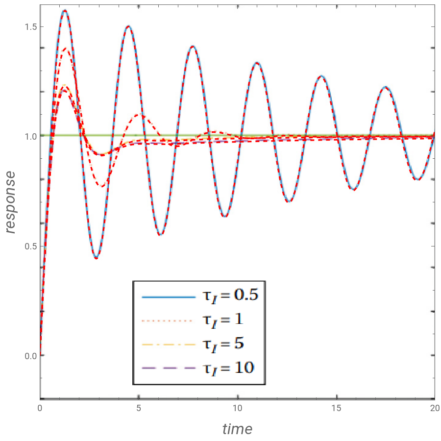
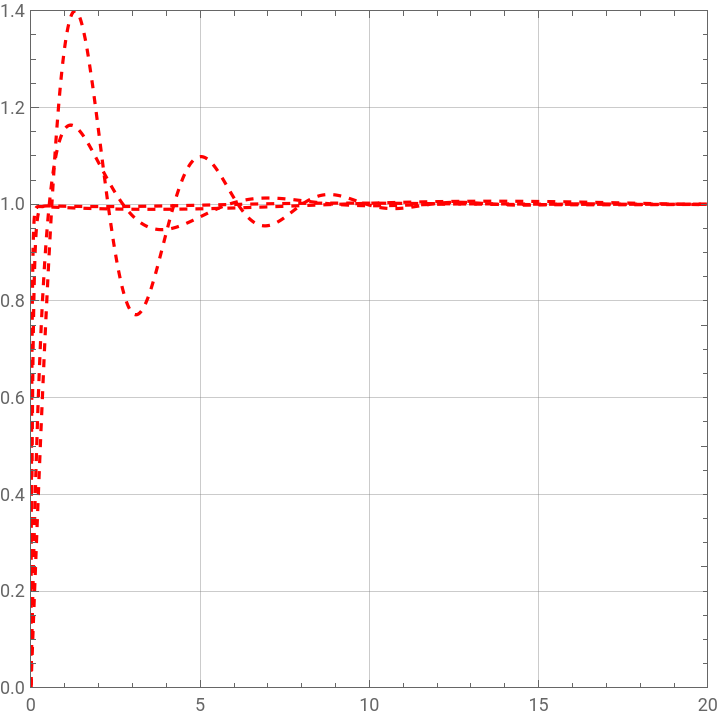
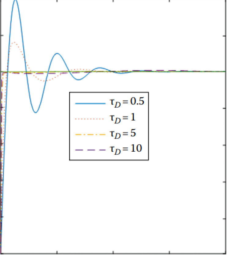
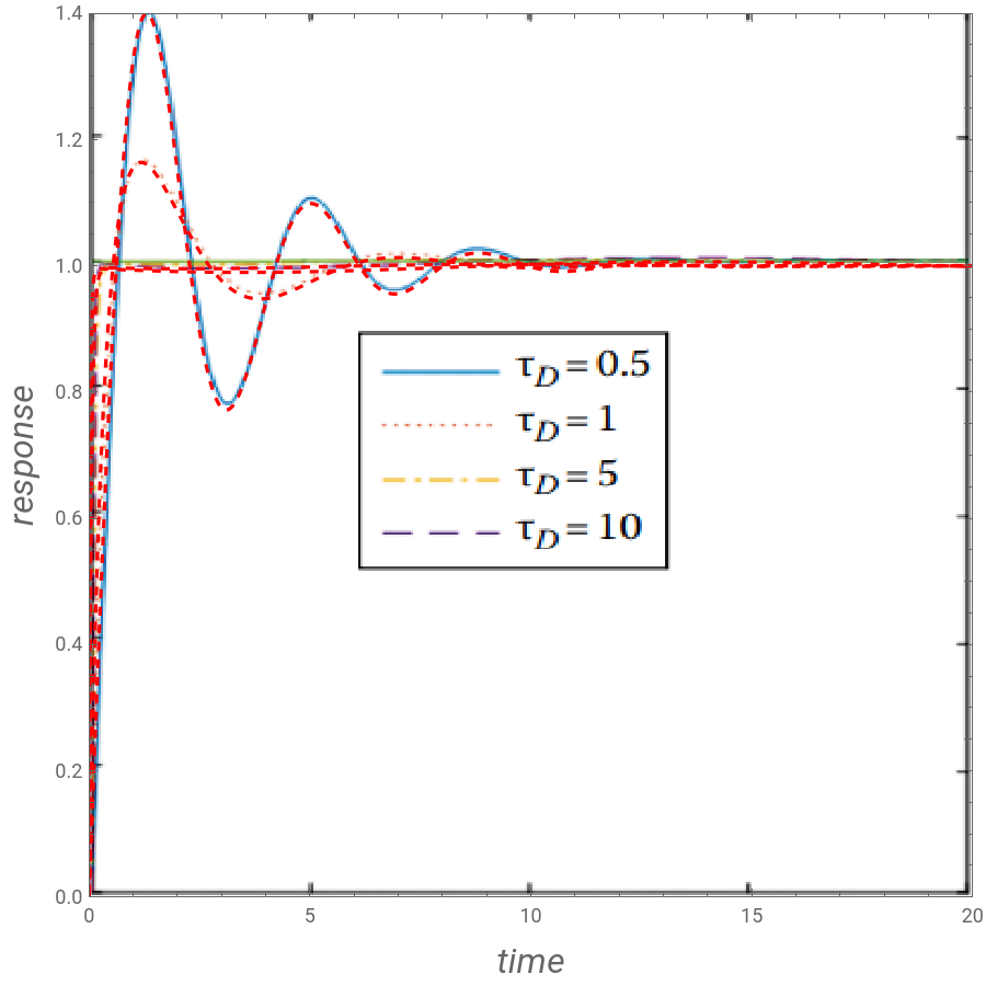
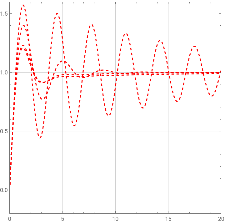
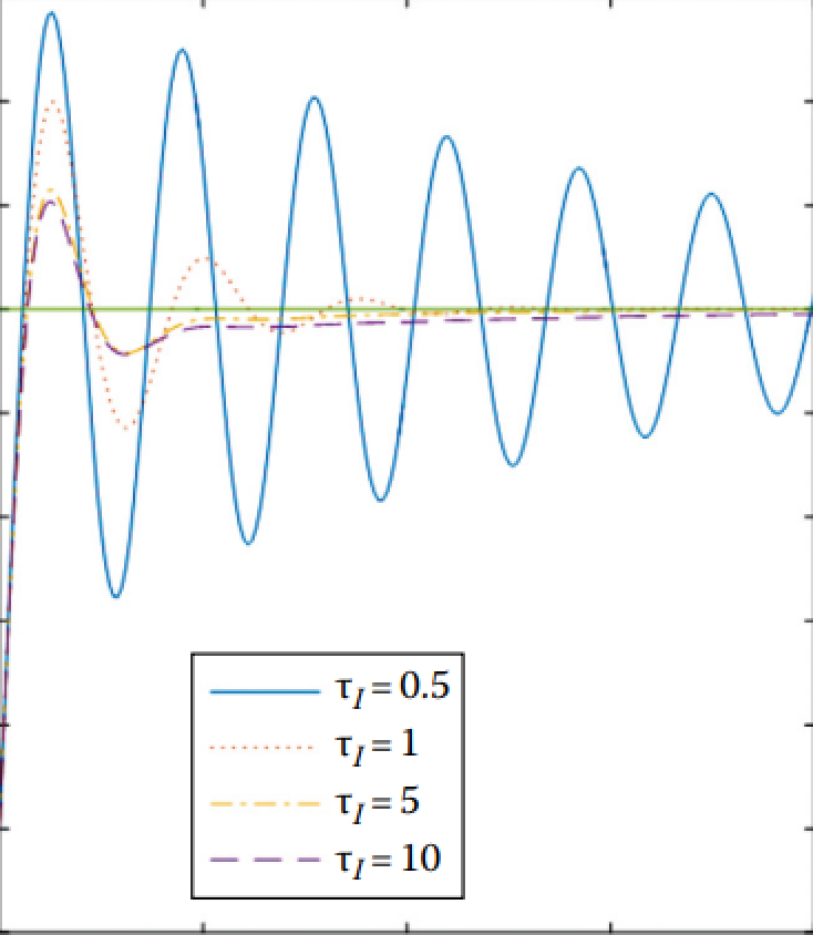
Figure below shows a simple feedback control system where the process transfer function is Gp(s) = 3/(4 s^2 + s + 1) and the proportional–integral–derivative (PID) controller is used. This controller transfer function is Gc(s) = Kc(1 + 1/(τI s) + τD s). We calculate and plot the closed-loop response to a unit step change in the set-point for various values of τI and τD while the value of Kc being kept constant equal to 5. Our results are superimposed to their counterpart given in Example 9.17 of Ref. 1.References:[1] Yeo, Yeong Koo, Chemical engineering computation with MATLAB, Boca Raton : Taylor & Francis, CRC Press, 2017.

In[]:=
Gp=3/(4s^2+s+1)
Out[]=
3
1+s+4
2
s
In[]:=
Gc[i_]:=Kc(1+1/s/tauI[[i]]+tauD[[i]]s)
In[]:=
GFBLOOP[i_]:=Gc[i]Gp/(1+Gc[i]Gp)//FullSimplify
In[]:=
Kc=5;tauI={1,1,1,1};tauD={0.5,1,5,10};
In[]:=
invLP=Table[InverseLaplaceTransform[GFBLOOP[i]1/s,s,t],{i,1,4}];
In[]:=
p=Plot[invLP,{t,0,20},PlotRange{{0,20},{0,1.4}},FrameTrue,GridLinesAutomatic,AspectRatio1,PlotStyle{{Red,Dashed},{Red,Dashed},{Red,Dashed},{Red,Dashed}}]
Out[]=
In[]:=
IMG=
;
In[]:=
Show[p,ImageSize450{1,1},Prolog{Raster[ImageData[IMG,DataReversedTrue],{Scaled[{0.0,0.0}],Scaled[{1,1.00}]}]},FrameLabel{Style["time",16,Italic],Style["response",16,Italic]}]
Out[]=
In[]:=
Kc=5;tauD=0.5{1,1,1,1};tauI={0.5,1,5,10};
In[]:=
invLP=Table[InverseLaplaceTransform[GFBLOOP[i]1/s,s,t],{i,1,4}];
In[]:=
p=Plot[invLP,{t,0,20},PlotRange{{0,20},{-0.2,1.6}},FrameTrue,GridLinesAutomatic,AspectRatio1,AxesOrigin{0,-0.2},PlotStyle{{Red,Dashed},{Red,Dashed},{Red,Dashed},{Red,Dashed}}]
Out[]=
In[]:=
IMG=
;
In[]:=
Show[p,ImageSize450{1,1},Prolog{Raster[ImageData[IMG,DataReversedTrue],{Scaled[{0.0,0.0}],Scaled[{1,1.00}]}]},FrameLabel{Style["time",16,Italic],Style["response",16,Italic]}]
Out[]=