I agree with your comments completely. The accumulated case data represent a serially dependent function but that is why it is modeled with a differential equation. Tomorrow’s new case count is a function of the number of actively infected cases today. It is also a function of the number of people exposed to the cases, the susceptibility of those people, the rate of transmission of the infection, and late in the process the number of people with immunity. There are sophisticated epidemiologic differential equations to deal with all the variables. However at this stage of the epidemic not enough is known about the disease process to use those equations without a lot of assumptions which may not be true.
The functions I presented will not likely be accurate until there are accumulated cases for more than one incubation period for the disease, and probably past the peak. The China data show that the fit improves progressively, with the growth rate, k, starting out high and later stabilizing around the current value. The L parameter may not have stabilized yet. So caution is advised.
The functions I presented will not likely be accurate until there are accumulated cases for more than one incubation period for the disease, and probably past the peak. The China data show that the fit improves progressively, with the growth rate, k, starting out high and later stabilizing around the current value. The L parameter may not have stabilized yet. So caution is advised.
For the sake of discussion, and perhaps to stimulate more people to contribute, let me present some evidence that supports the model.
First we need the cleanest data set we can get with sufficiently large numbers to be accurate. For this I have selected the China data, excluding the provinces of Hubei, and Shandong, where there are obvious irregularities. These cases were confirmed by laboratory testing, hopefully along the their contacts and even more hopefully accumulated in timely and orderly fashion. The data extraction functions are below in the next cell.
Data Extraction
The plots below show the sigmoid shape of the data vs time in days and that the first differences rise and fall; the new cases per day are currently at a much lower level than they were at the peak, suggesting that the epidemic is coming to an end.
In[]:=
ListPlot[selectCases]ListPlot[Differences@selectCases[[All,2]]]
Out[]=
Out[]=
Next we look for evidence that the data contain information consistent with the logistic model differential equation below.
f'[t]kf[t](1-f[t]/L)
In[]:=
deModel=kx1-
x
L
Out[]=
kx1-
x
L
Note that this is a quadratic function. x is now the accumulating number of cases. The equation has roots at zero and L, and its peak value is at L/2.
In[]:=
ddeModel=D[deModel,x]//ExpandAll;Solve[deModel0,x]Solve[ddeModel0,x]
Out[]=
{{x0},{xL}}
Out[]=
x
L
2
To look at this function from the data we need to calculate the first derivative with respect to time at each point. We create an interpolation function to do this.
In[]:=
selectFn=Interpolation[selectCases];selectDE={selectFn[#],selectFn'[#]}&/@Range[Length@selectCases];selectDEPlot=ListPlot[selectDE,PlotStyle->Darker@Red,GridLinesAutomatic,PlotRangeAll];deNLM=NonlinearModelFit[selectDE,deModel,{k,L},x];Show[Plot[deNLM[x],{x,0,L/.deNLM@"BestFitParameters"},PlotRangeAll,PlotLabel"Logistic Difference Equation"],selectDEPlot]
Out[]=
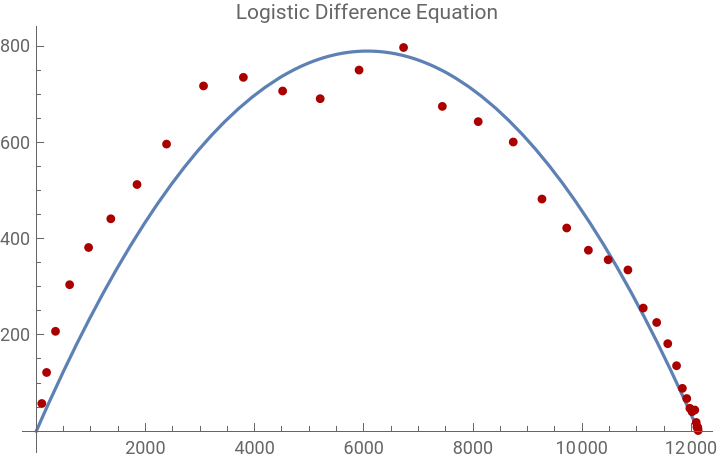
If you can accept that the data points in red indeed can be modeled by the quadratic equation in blue, then you will probably agree the model is good. The late data points look like they are becoming more accurate, and it looks like the epidemic in China outside the excluded provinces should be coming to an end quite soon.
In[]:=
deNLM@"BestFitParameters"selectNLM=NonlinearModelFitselectCases,L(1+),{{k,0.3},{L,15000},{t0,20}},t;selectNLM@"BestFitParameters"
-k(t-t0)
Out[]=
{k0.260473,L12128.}
Out[]=
{k0.264631,L12094.6,t013.3109}
Above are the data fits by each method--they are quite close. To get t0, we find the solution where the data function, selectFn[t0] == L/2.
In[]:=
FindRoot[selectFn[t0]L/2/.deNLM["BestFitParameters"],{t0,20}]
Out[]=
{t013.1884}