This essay analyzes the relationship between model capacity and the flatness of minimizers across the double descent curve. Using filter-normalized loss surface visualizations, we find that the minimizer is the sharpest at the interpolation threshold and becomes gradually flatter as capacity moves in either direction—toward the under-parameterized sweet spot or deeper into the over-parameterized regime.
Many Many Parameters—Which Solution is Found by Descent?
Many Many Parameters—Which Solution is Found by Descent?
Deep learning’s success relies on training over-parameterized neural networks with far more parameters than available data points. Their loss function therefore lives in a very high-dimensional space where there are many local minimizers with similar loss values. Surprisingly, gradient descent consistently finds solutions that generalize well to unseen data. Understanding which solution is found by gradient descent, and why certain solutions generalize better than others remains a central question in deep learning research. This essay examines two key phenomena that shed light on this question. First, the geometry of the loss landscape—specifically, whether gradient descent converges to sharp or flat minimizers—appears to influence generalization. Second, the double descent phenomenon reveals that increasing model capacity beyond the interpolation threshold unexpectedly improves generalization.
Double Descent
Double Descent
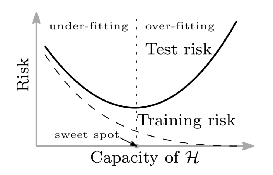
Double descent describes the relationship between model capacity and test risk observed in modern neural network models with high model capacity. Classically, the relationship between the model capacity and its test error is described by a U-shaped curve from the bias-variance trade-off, where if the model capacity is too small, the model under-fits the training data (i.e., large training error and test error) and if the capacity is too large, the model over-fits the training data (i.e., small training error but large test error). The following figure, from Belkin et al. (2019), shows the U-shaped bias-variance trade-off curve.
However, modern machine learning models such as deep neural networks contradict the bias-variance trade-off. These rich models are often trained to exactly fit the training data to achieve a near-zero training error. The point where the training error becomes approximately zero is called the “interpolation threshold.” However, despite their high model capacity and near-perfect fit to the data, they also retain a very high accuracy on test data, contradicting our classical understanding. Belkin et al. (2019) formulated the “double descent curve” which includes the U-shaped curve and extends it beyond the interpolation threshold, as shown below.
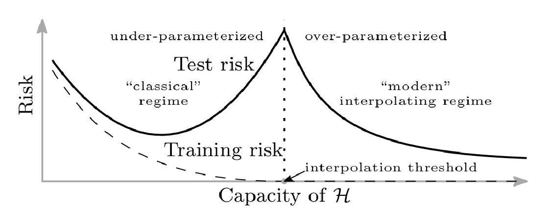
Below the interpolation threshold (i.e., the “classical” regime), the test risk follows the traditional U-shaped curve, and the test risk peaks at the interpolation threshold. Above the interpolation threshold (i.e., the “modern” interpolating regime), the test risk decreases as the model capacity increases. Nakkiran et al. (2019) provide extensive empirical evidence for the double descent phenomenon across modern deep learning architectures (ResNets, CNN, Transformers) and datasets (CIFAR-10, CIFAR-100, IWSLT14). Their experiments reveal that the test error peak occurs at the interpolation threshold across various settings, confirming that models with capacity sufficiently beyond this threshold achieve better generalization than those in the under-parameterized regime.
The Flat Minima Hypothesis
The Flat Minima Hypothesis
The flat minima hypothesis posits that the local curvature of the minimizers found by gradient descent affects generalization of a neural network. Hochreiter & Schmidhuber (1997) first proposed that flat minimizers, characterized by low curvature, lead to better generalization than sharp minimizers. Keskar et al. (2017) formalize this distinction between sharp and flat minimizers through local curvature properties and Hessian eigenvalues. Sharp minimizers are characterized by a significant number of large positive eigenvalues in f(x) while flat minimizers have numerous small eigenvalues in f(x), indicating low curvature across many directions. The following is a conceptual sketch of flat and sharp minimizers, from Keskar et al. (2017), where the y-axis indicates the loss value and x-axis represents the parameters.
2
∇
2
∇
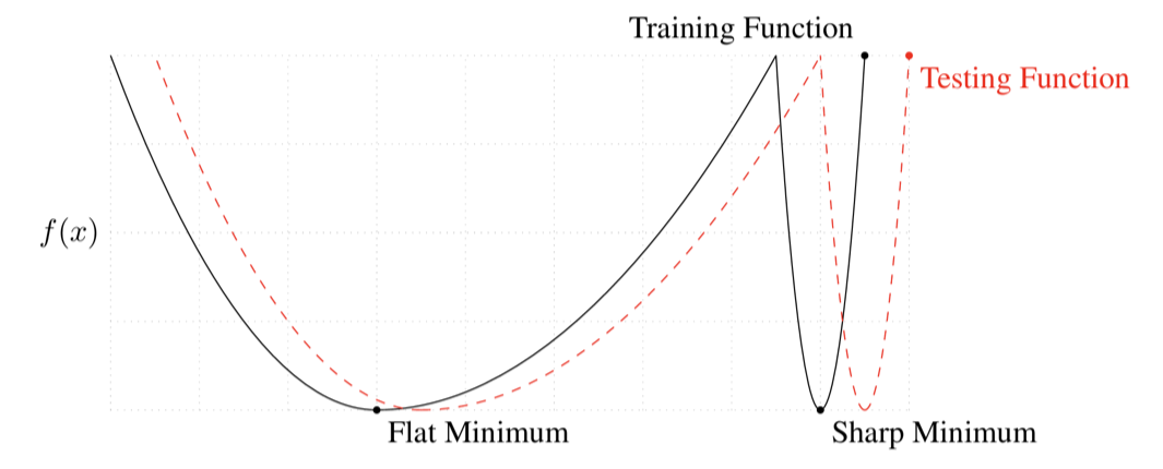
As can be seen in the figure above, a flat minimizer exhibits slow variation of the loss function in a relatively large neighborhood of parameters, and thus can be described with lower precision, while a sharp minimizer shows rapid increase within a small neighborhood. Keskar et al. (2017) connect this to the Minimum Description Length (MDL) Principle, the idea that models with lower descriptive complexity like the flat minimizers generalize better.
The Research Question
The Research Question
Although the flat minima hypothesis and the double descent phenomena are well-studied independently, their connection remains unclear. In this essay, we explore the following question: What is the relationship between model capacity and loss landscape geometry across the double descent curve?”
Constructing the Experiment
Constructing the Experiment
To explore the loss landscape geometry across the double descent curve, we reproduce the convolutional neural network experiments from Nakkiran et al. (2019). We follow their experimental setup in which model-wise double descent was observed; see Nakkiran et al. (2019) for complete details.
Dataset
Dataset
Following Nakkiran et al. (2019), we use CIFAR-10 without data augmentation.
Retrieving the dataset information
In[]:=
ResourceObject["CIFAR-10"]
Out[]=
ResourceObject


Importing the training data
In[]:=
trainingData=ResourceData["CIFAR-10","TrainingData"];
Importing the training data
In[]:=
testData=ResourceData["CIFAR-10","TestData"];
Defining a label encoder for class labels
In[]:=
labelEncoder=NetEncoder[{"Class",{"airplane","automobile","bird","cat","deer","dog","frog","horse","ship","truck"},"IndicatorVector"}]
Out[]=
NetEncoder
One-hot encoding the training data class labels
In[]:=
trainingData=#[[1]]->labelEncoder[#[[2]]]&/@trainingData;
One-hot encoding the test data class labels
In[]:=
testData=#[[1]]->labelEncoder[#[[2]]]&/@testData;
Model Architecture
Model Architecture
We train 5-layer convolutional neural networks following the architecture described in Nakkiran et al. (2019), consisting of Conv-BatchNorm-ReLU-MaxPool blocks followed by a max-pooling layer and a fully-connected output layer. The four convolutional layers have filters respectively, where the width parameter controls the model capacity. Varying allows us to systematically explore the under-parameterized, critical, and over-parameterized regimes. The PyTorch specification of their CNNs is available at https://gitlab.com/harvard-machine-learning/double-descent/tree/master.
[k,2k,4k,8k]
k
k
Defining the Conv-BatchNorm-ReLU-MaxPool block
In[]:=
convBlock[n_Integer,k_Integer,w_Integer]:=Module[{filterSize=n*k},NetChain[{ConvolutionLayer[filterSize,{3,3},"Stride"->1,"PaddingSize"->1],BatchNormalizationLayer["Epsilon"->0.00001,"Momentum"->0.1],ElementwiseLayer["ReLU"],PoolingLayer[w,w,"Function"->Max]}]]
First, we compute the mean and variance of the training data to normalize it.
Obtain the image data in a tensor form
In[]:=
imageTensor=ImageData[#[[1]]]&/@trainingData;
Compute the means for each image channel
In[]:=
meanlist=Table[Mean[Flatten[imageTensor[[;;,;;,i]]]],{i,1,3}]
Out[]=
{0.489006,0.479704,0.476805}
Compute the variances for each image channel
In[]:=
varlist=Table[Variance[Flatten[imageTensor[[;;,;;,i]]]],{i,1,3}]
Out[]=
{0.0700036,0.0670789,0.0657609}
Constructing the network architecture
In[]:=
convNet[k_Integer]:=NetInitialize[NetChain[<|"Conv1"->convBlock[1,k,1],"Conv2"->convBlock[2,k,2],"Conv3"->convBlock[4,k,2],"Conv4"->convBlock[8,k,2],"Pool4"->PoolingLayer[4,4,"Function"->Max],"FC_Output"->LinearLayer[10],"Softmax"->SoftmaxLayer[]|>,"Input"->NetEncoder[{"Image",{32,32},"MeanImage"->meanlist,"VarianceImage"->varlist}]],Method->{"Kaiming","Distribution"->"Uniform"}]
Label Noise
Label Noise
Following Nakkiran et al. (2019), we inject 20% label noise into the training data by randomly replacing labels with uniformly sampled incorrect classes. The authors observe double descent most strongly in settings with label noise, noting that the test error peak becomes “more prominent in settings with label noise” (Nakkiran et al., 2019).
Function for adding (p×100)% noise to the data
In[]:=
addLabelNoise[x_,p_Real]:=Module[{data=x,n=Floor[p*Length[x]],ind=List[],labels=IdentityMatrix[10],trueLabels=List[],corruptedLabels=List[]},ind=RandomInteger[{1,Length[data]},n];trueLabels=data[[ind,2]];corruptedLabels=RandomChoice[Delete[labels,FirstPosition[#,1]]]&/@trueLabels;data[[ind,2]]=corruptedLabels;Return[data]]
Adding 20% label noise to the training data
The specific set of noisy labels used for the experiment is provided below for reproducibility
Training the Neural Networks
Training the Neural Networks
Function for training a CNN with width parameter k
Association for storing the networks
Training and saving the network parameters
Double Descent Curve
Double Descent Curve
Evaluating the Network Performance
Evaluating the Network Performance
Computing the test error rates
Computing the training error rates
Visualizing the Double Descent Curve
Visualizing the Double Descent Curve
Plotting both test and training error rates against the model width parameter k results in the characteristic double descent curve.
Analysis
Analysis
The experimental results can be interpreted through the double descent framework introduced by Belkin et al. (2019). Two regimes emerge, separated by the interpolation threshold.
These two regimes will serve as the basis for comparing loss landscape geometry in subsequent sections.
Loss Surface Visualization Methods
Loss Surface Visualization Methods
Precisely measuring the sharpness of a minimizer poses a challenge. Keskar et al. (2017) characterize flatness using eigenvalues of the Hessian. However, Dinh et al. (2017) demonstrated that such measures are not invariant to the symmetries inherent in rectified networks. That means simple reparameterization can arbitrarily change the measured sharpness without actually affecting the model behavior. In other words, multiplying one layer by α and dividing the next layer by α does not change the model behavior, but can change the measured sharpness. Li et al. (2018) addressed this through filter-normalization, which mitigates the scaling effect and enables more meaningful comparisons of different minimizers by producing visualizations where sharpness correlates well with generalization error.
Random Directions Plot
Random Directions Plot
Function that produces random direction vectors sampled from Gaussian distribution
Following Li et al. (2018), the batch normalization parameters are held constant.
Layers perturbed by random directions
Cross-entropy loss function
Function for visualizing of the loss surface of local minimizers using a random directions plot
Filter-Normalization
Filter-Normalization
Function for computing the Frobenius norm of a convolutional filter or a linear layer weight matrix
Normalizing each filter
Function for Finding Filter Normalized Directions
Filter-Normalized Plots
Filter-Normalized Plots
Association for storing the filter-normalized loss surface plots
Creating filter-normalized loss surface plots for networks with different width parameters
Results
Results
The loss surface plots are presented below, organized into each regime along the double descent curve.
Analysis and Discussion
Analysis and Discussion
Limitations and Future Directions
Limitations and Future Directions
This essay’s analysis was limited to qualitative measures of sharpness through filter-normalized visualizations. Although filter normalization is empirically shown to produce results that correlate well with generalization performance, the qualitative analysis is limited to explorative purposes. For a more robust analysis, future work could employ quantitative measures of sharpness, such as Hessian eigenvalues.
Our experiments used a single architecture (5-layer CNN) and dataset (CIFAR-10). Extending this analysis to other architectures (e.g., ResNets, Transformers) and datasets would test the generality of our findings. Finally, while we observed that over-parameterized models converge to flatter minimizers, the mechanism behind this phenomenon is not explored. Investigating why gradient descent finds flatter minimizers as model capacity increases would be a worthwhile future research direction.
References
References
◼
Belkin, M., Hsu, D., Ma, S., & Mandal, S. (2019). Reconciling modern machine-learning practice and the classical bias–variance trade-off. Proceedings of the National Academy of Sciences, 116(32), 15849–15854. doi:10.1073/pnas.1903070116
◼
Dinh, L., Pascanu, R., Bengio, S., & Bengio, Y. (2017). Sharp Minima Can Generalize For Deep Nets. arXiv [Cs.LG]. Retrieved from http://arxiv.org/abs/1703.04933
◼
Hochreiter, S., & Schmidhuber, J. (01 1997). Flat Minima. Neural Computation, 9(1), 1–42. doi:10.1162/neco.1997.9.1.1
◼
Keskar, N. S., Mudigere, D., Nocedal, J., Smelyanskiy, M., & Tang, P. T. P. (2017). On Large-Batch Training for Deep Learning: Generalization Gap and Sharp Minima. arXiv [Cs.LG]. Retrieved from http://arxiv.org/abs/1609.04836
◼
Li, H., Xu, Z., Taylor, G., Studer, C., & Goldstein, T. (2018). Visualizing the Loss Landscape of Neural Nets. arXiv [Cs.LG]. Retrieved from http://arxiv.org/abs/1712.09913
◼
Nakkiran, P., Kaplun, G., Bansal, Y., Yang, T., Barak, B., & Sutskever, I. (2019). Deep Double Descent: Where Bigger Models and More Data Hurt. arXiv [Cs.LG]. Retrieved from http://arxiv.org/abs/1912.02292
CITE THIS NOTEBOOK
CITE THIS NOTEBOOK
Loss landscape geometry across the double descent curve
by Junseo Lee
Wolfram Community, STAFF PICKS, January 10, 2026
https://community.wolfram.com/groups/-/m/t/3603794
by Junseo Lee
Wolfram Community, STAFF PICKS, January 10, 2026
https://community.wolfram.com/groups/-/m/t/3603794