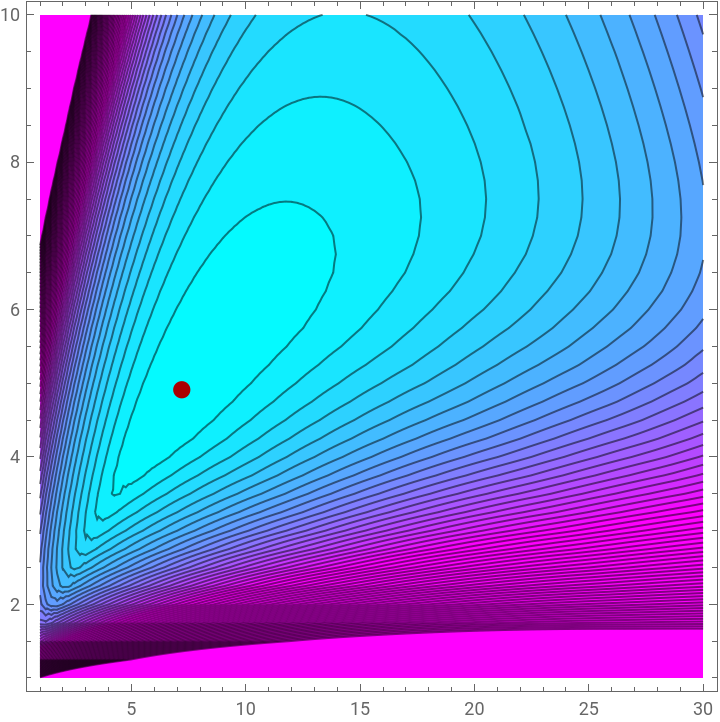
PI Controller Tuning : Contour plots of ISE, IAE and ITAE
Authors: Housam Binous and Ahmed Bellagi
PI Controller Tuning : Contour plots of ISE, IAE and ITAE
Authors: Housam Binous and Ahmed Bellagi
Authors: Housam Binous and Ahmed Bellagi
MATHEMATICA code below uses NMINIMIZE to fetch best PI controller parameters. To do so it employs the ISE, IAE or the ITAE criteria. The MATHEMATICA command Parallelize is used in order to reduce computation time.
In[]:=
Gc[KP_?NumericQ,TAUI_?NumericQ]:=KP+TAUI/s;GT=1/(s+1)/(s+2)/(s+3)
Out[]=
1
(1+s)(2+s)(3+s)
In[]:=
G[KP_?NumericQ,TAUI_?NumericQ]:=GTGc[KP,TAUI]/(1+GTGc[KP,TAUI])
In[]:=
y[KP_?NumericQ,TAUI_?NumericQ]:=InverseLaplaceTransform[1/sG[KP,TAUI],s,t]//Chop;
ISE CRITERIA
In[]:=
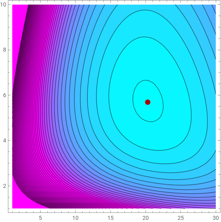
f1[KP_?NumericQ,TAUI_?NumericQ]:=Re[Quiet@NIntegrate[(1-y[KP,TAUI])^2,{t,0,30}]//Chop];
In[]:=
NMinimize[f1[KP,TAUI],{KP,TAUI},MaxIterations->10]
Out[]=
{0.696163,{KP20.2936,TAUI5.69173}}
In[]:=
LaunchKernels[]
Out[]=
KernelObject,KernelObject,KernelObject,KernelObject

In[]:=
data=Parallelize@Table[{KP,TAUI,f1[KP,TAUI]},{KP,1,30,0.25},{TAUI,1,10,0.25}]
Out[]=
In[]:=
CoolColor[z_]:=RGBColor[10z,1-10z,1];
In[]:=
p1=ListContourPlot[Flatten[data,1],Contours->Join[Table[i0.1,{i,0,20,0.25}]],PlotRange->All,ColorFunctionCoolColor];
In[]:=
Show[p1,Graphics[{Darker@Red,PointSize[0.025],Point[{KP,TAUI}/.{KP->20.2936,TAUI->5.69173}]}],PlotLegendsAutomatic]
Out[]=
IAE CRITERIA
In[]:=
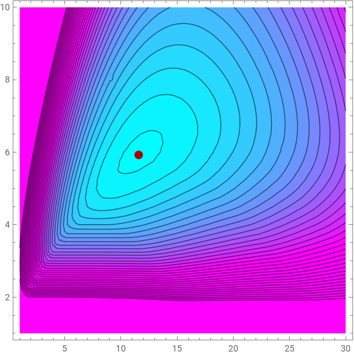
f2[KP_?NumericQ,TAUI_?NumericQ]:=Re[Quiet@NIntegrate[Abs[(1-y[KP,TAUI])],{t,0,30}]//Chop];
In[]:=
NMinimize[f2[KP,TAUI],{KP,TAUI},MaxIterations->10]
Out[]=
{1.28735,{KP11.5836,TAUI5.92557}}
In[]:=
data2=Parallelize@Table[{KP,TAUI,f2[KP,TAUI]},{KP,1,30,0.25},{TAUI,1,10,0.25}]
Out[]=
In[]:=
p2=ListContourPlot[Flatten[data2,1],Contours->Join[Table[i0.1,{i,0,30,0.5}]],PlotRange->All,ColorFunction->CoolColor];
In[]:=
Show[p2,Graphics[{Darker@Red,PointSize[0.025],Point[{KP,TAUI}/.{KP->11.5836,TAUI->5.92557}]}]]
Out[]=
IAE CRITERIA
In[]:=
f3[KP_?NumericQ,TAUI_?NumericQ]:=Re[Quiet@NIntegrate[tAbs[(1-y[KP,TAUI])],{t,0,30}]//Chop];
In[]:=
NMinimize[f3[KP,TAUI],{KP,TAUI},MaxIterations->10]
Out[]=
{1.52357,{KP7.19957,TAUI4.91172}}
In[]:=
data3=Parallelize@Table[{KP,TAUI,f3[KP,TAUI]},{KP,1,30,0.25},{TAUI,1,10,0.25}]
Out[]=
In[]:=
p3=ListContourPlot[Flatten[data3,1],Contours->Join[Table[i,{i,0,30,0.5}]],PlotRange->All,ColorFunction->CoolColor];
In[]:=
Show[p3,Graphics[{Darker@Red,PointSize[0.025],Point[{KP,TAUI}/.{KP->7.19957,TAUI->4.91172}]}]]
Out[]=