Statement of the Problem
Statement of the Problem
In[]:=
<<MaTeX`
In[]:=
Out[]=

One-liner Solution
One-liner Solution
At the first glance it seems very challenging because depends on its own integral. So either we need differential equation or some reclusive method, which is hoax. By definition of definite integral, we notice the integral of over interval is a real positive constant instead of antiderivative. Let’s assume the integral is . Therefore, We have an expression of . The problem is reduced to find the solution of the following equation, which is the only critical step using one line:
f(x)
f(t)
[0,1]
a>0
f(x)
In[]:=
sol=Solve[Integrate[RealAbs[x^3-4*x*a],{x,0,1}]a,a]
Out[]=
a,a
1
8
1
4
Once is determined, the following steps are just cutting butter with hot knife. we define the functions:
a
In[]:=
f1[x_]:=x^3-4*x*1/8
In[]:=
f2[x_]:=x^3-4*x*1/4
Visualize the functions and their counterpart with absolute value over a symmetric domain:
In[]:=
{Plot[Evaluate[{f1[x],f2[x]}],{x,-1,1},PlotLegends"Expressions"],Plot[Evaluate[RealAbs@{f1[x],f2[x]}],{x,-1,1},PlotLegends"Expressions"]}//Column
Out[]=


The local maximum values can be found with the build-in optimization function with the visualization above:
In[]:=
Maximize[{#[x],x<0},x]&/@{f1,f2}
Out[]=
,x-,,x-
1
3
6
1
6
2
3
3
1
3
We can also quickly check the result:
In[]:=
f1[x]===(x^3-4*x*Integrate[RealAbs@f1[x],{x,0,1}])
Out[]=
True
In[]:=
f2[x]===(x^3-4*x*Integrate[RealAbs@f2[x],{x,0,1}])
Out[]=
True
Analysis
Analysis
The basic idea is quite similar to the one liner solution. To understand better what is behind the automation, we can break down the code a little bit. Using the same definition for variable , we can take a look at the LHS of our equation
a
In[]:=
Simplify[Integrate[RealAbs[x^3-4*x*a],{x,0,1}],Assumptionsa>0]
Out[]=
|
Mathematica automatically converts the integral in to a piecewise function of . Fantastic! The geometric interpretation is as simple as to find the intersection between the curve of identity function and the piecewise function.
a
In[]:=
Plot
,a,{a,0,1/3},AspectRatio1,EpilogPoint[{a,a}/.sol],PlotLegendsPlaced[{"Piecewise","f(a) = a"},Above]
|
Out[]=
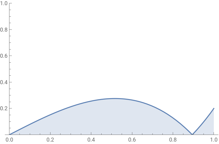
Using the following active demonstration we shall see why we need to consider the equation over separate domains for . Simple algebra tells us that the root of is }. Thus if the positive root is on the right hand side of , we can integrate the directly. Otherwise, we have to do integral on two domains for : use from and from .
a
f(x)
{-2
a
,0,2a
x=1
f(x)
f(x)
f(x)
{0,2
a
}-f(x)
{0,2
a
}In[]:=
ListAnimate[Table[Plot[RealAbs[x^3-4*x*a],{x,0,1},FillingAxis,PlotRange{0,1}],{a,0.05,0.45,0.05}]]
Out[]=
Remark
Remark
◼
Use definition of definite integral to find the algebraic expression of the given function
◼
Convert the form the given function to algebraic equation
◼
Find relationship between the definite integral and the location of the root of the given function
◼
Use symmetry and monotonicity of cubic function based on root location to find local maximum