This project constructs a graph based on the positions of a sample of galaxies. The data of the galaxies is available, it contains 133 991 galaxies distributed roughly in the sky region 100<RA<270 and −7<DE<65. The data can be obtained as a Cloud object, but also data can be obtained directly from the Vizier database with the preliminary function AstroCatalogData. Using the data, some general aspects of it are discussed, as the distance to k nearest neighbor. Then, some clustering ideas using the Wolfram Language capabilities are discussed. Finally, a method to construct a graph from the data is presented.
The Data
The Data
This project takes data from the catalog SDSS NASA/AMES Value Added Galaxy Catalog , specifically from the “table8.dat” file. This file contains information of galaxies distributed roughly in the sky region 100<RA<270 and −7<DE<65. Initially, the data comes from measurements of the Sloan Digital Sky Survey (SDSS) Data Release 7. This data can be obtained using the preliminary function AstroCatalogData, which download tables of data from the the Vizier database.
AstroCatalogData uses the python package astroquery, then before using this function you must have Python running from Mathematica with the packages numpy, pandas, and astroquery. I recommend using the functions FindPythonExecutable and PythonPackageInstall, which do these things automatically. Once AstroCatalogData is ready to run you can get the data as (check the documentation to see how AstroCatalogData works):
(AMES–VAGC)
AstroCatalogData uses the python package astroquery, then before using this function you must have Python running from Mathematica with the packages numpy, pandas, and astroquery. I recommend using the functions FindPythonExecutable and PythonPackageInstall, which do these things automatically. Once AstroCatalogData is ready to run you can get the data as (check the documentation to see how AstroCatalogData works):
In[]:=
AstroCatalogData=ResourceFunction[CloudObject[
https://www.wolframcloud.com/obj/truman.tapia/DeployedRe
sources/Function/AstroCatalogData
]]Out[]=
In[]:=
AstroCatalogData["J/ApJ/799/95/table8","Columns"All]
Out[]=
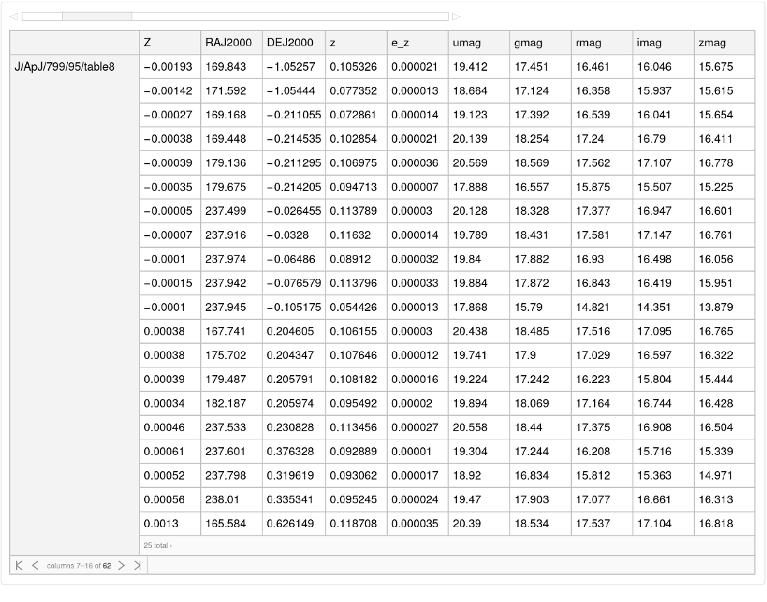
According to Way et al. (2015), before using this data one needs to remove the galaxies that fail the tests 55’’ Fiber Placement Issue and Flagging Boundary Points, the failing galaxies are specified in the same dataset (more information about the data can be found here). After removing the galaxies that complain with these tests, one ends with the information of galaxies. The cleaned data join with cartesian coordinates in megaparsecs Mpc of each galaxy can be obtained as:
133991
In[]:=
data=CloudImport[CloudObject["https://www.wolframcloud.com/obj/truman.tapia/galaxydata"]]
Out[]=
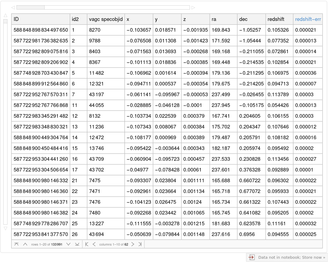
here each row is a galaxy and each column is a field of information. The most important piece of information for this work are the last three columns, which are the added cartesian coordinates.
Little aspects about the distribution of galaxies
Little aspects about the distribution of galaxies
Once the coordinates of thousands of galaxies are available, one could just plot them to try to see how the Universe looks like as natural as possible
In[]:=
coordinates=Values@Normal[data[All,{"xphy","yphy","zphy"}]];xmin=data[Min,"xphy"];xmax=data[Max,"xphy"];ymin=data[Min,"yphy"];ymax=data[Max,"yphy"];zmin=data[Min,"zphy"];zmax=data[Max,"zphy"];
In[]:=
ColorConvert[Quiet@ListPointPlot3D[coordinates,DataRange{Full,Full,Full},BoxedFalse,Axes->False,BoxRatios{1,1,1},ViewPoint{.4,.7,.8},PerformanceGoal"Speed"],"CMYK"]
Out[]=
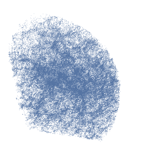
It immediately jumps the foam like structure of the Universe. Also, it can be important to know the distribution of the galaxies according to their position in the cartesian coordinates, here plotted as a histogram the distribution of galaxies according to their x, y, and z coordinates in Mpc.
In[]:=
Histogram/@{coordinates〚All,1〛,coordinates〚All,2〛,coordinates〚All,3〛}
Out[]=

Another interesting measurement could be the distribution of distances to the k nearest neighbor in the hole dataset; here presented the distribution to the first, second, and third nearest neighbor respectively:
In[]:=
galaxyDists[list_]:=Map[Norm,coordinates-list]galaxiesknearest[k_]:=With[{splitNearest=(Nearest[coordinates,coordinates,k+1]〚All,#+1〛&/@Range[k])},Map[galaxyDists,splitNearest]]n=galaxiesknearest[20];Histogram[#,{.2}]&/@n[[;;3]]
Out[]=

Obviously the maximum of the distribution is going to move to the right (increase) as the k nearest neighbor increases; following the distance to the 101, 102, and 103 nearest neighbor distributions:
n=galaxiesknearest[103];Histogram[#,{1}]&/@n[[;;3]]
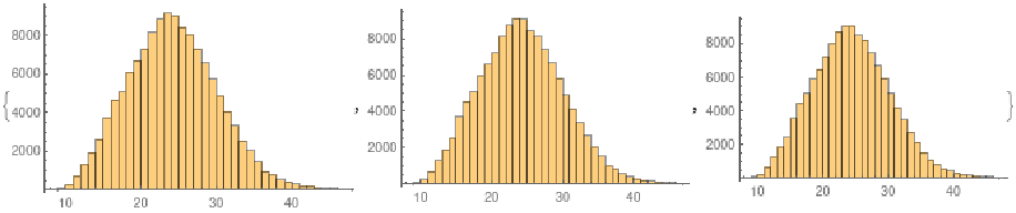
All the distributions except for the first few ones present the same shape.
Clustering
Clustering
Seeing the first figure of this work one cannot say much about the structure of the Universe, then some clustering work is needed to understand the Large Scale Structure (LSS). The clustering capabilities of the Wolfram Language certainly can be useful in this task. Following the function FindClusters with the spanning tree method is tested with several pruning distances (called MaxEdgeLength in the function). First, a minibox inside the dataset is created to test this clustering approach:
Then, the FindCluster function is used with several MaxEdgeLength, and then the number of clusters is extracted:
One may expect the number of clusters is going to increase as the MaxEdgeLength gets smaller, but this is not the case, which suggest some difficulties for this function to properly cluster the galaxies. The documentation of the SpanningTree (as some other methods) mention that: “it can fail when clusters have different densities or are loosely connected.”
Another clustering criterion can be to use the function LearnDistribution to get a probability density estimate of the hole space of the dataset, and then cluster structures with high density estimate (this has been done in many works about the LSS). This time I work with this smaller box inside the space of the dataset:
And the distribution function is:
The resulting LearnedDistribution uses the method KernelDensityEstimation, which is a classical method in LSS works. Then, the resulting PDF profile of the distribution along with the point galaxies (in red) is:
It is clear that some kind of clustering arises using this approach.
It is clear that some kind of clustering arises using this approach.
Graph Reconstruction
Graph Reconstruction
The main objective of this project is to construct a graph based on the LSS of the Universe. From the last image one could imaging that a 3D counterpart of the function MorphologicalGraph could be very useful to find a graph representation of the cosmic web. Since this counterpart does not exist (yet), one could try to make slices of the figure, but this could be computationally demanding. On the hand, one could say that there is no right answer in finding the structure of the Universe. In the paper Tracing the cosmic web, Libeskind et al. (2018) try 12 different algorithms to find structures in the LSS, and they conclude : “Each web finder captures different aspects of this very complex pattern...”. With this kind of freedom in mind (there is not fully right answer), following I construct a graph using a distance criterion to join galaxies and then construct clusters.
An undirected graph will be constructed using the position of galaxies as nodes and building edges between close galaxies. First a small box2 is constructed inside the space of the dataset, and the UndirectedEdge function gets the Orderless attribute to consider that a b is equal to b a:
An undirected graph will be constructed using the position of galaxies as nodes and building edges between close galaxies. First a small box2 is constructed inside the space of the dataset, and the UndirectedEdge function gets the Orderless attribute to consider that a b is equal to b a:
Then, an initialization function is implemented to target n galaxies in the box2 variable, and to build useful associations to go from targets to positions and vice versa:
Now, a function called miniweb that takes a node (nodo), a list of search (listOfSearch), and a distance (r); and returns a list of edges connecting the nodes than are closer than a distance r to nodo (the close nodes are search in the listOfSearch list):
The following two functions construct a cluster of galaxies joining galaxies using the miniweb function nestly:
Finally the function miniuniverse creates all the clusters that are possible in the sample of galaxies
Future works may include to study the properties of the emerging graphs, and of course finding new ways to reconstruct graphs from the cosmic web.
Acknowledgment
Acknowledgment
Mentor: John Cassel
Thank you for the great advices and support provided to make this work possible.
References
References
◼
Way, M. J., Gazis, P. R., & Scargle, J. D. (2015). Structure in the 3D galaxy distribution. II. Voids and watersheds of local maxima and minima. The Astrophysical Journal, 799(1), 95.
◼
Libeskind, N. I., Van De Weygaert, R., Cautun, M., Falck, B., Tempel, E., Abel, T., ... & Gottlöber, S. (2018). Tracing the cosmic web. Monthly Notices of the Royal Astronomical Society, 473(1), 1195-1217.