ABSTRACT (original article): A remarkable feat of active matter physics is that systems as diverse as collections of self propelled particles, nematics mixed with molecular motors and interacting robots can all be described by symmetry - based continuum theories. These descriptions rely on reducing complex effects of individual motors to a few key active parameters, which increase with activity. Here we observe a striking anomaly in the continuum description of nonreciprocal active solids, a ubiquitous class of active materials. Using a combination of metamaterial experiments and coarse - graining theory we find that as microscopic activity increases, macroscale active response can vanish: more is less. In this highly active regime, nonaffine and localized modes prevail and destroy the large - scale signature of microscopic activity. These modes exist in any dilute periodic structure and emerge in random lattices below a percolation transition. Our results unveil a counterintuitive facet of active matter, offering new principles for engineering materials far from equilibrium. CITATION (original article): Binysh, J., Baardink, G., Veenstra, J., Coulais, C., & Souslov, A. (2026). More is Less in Unpercolated Active Solids. Physical Review X. https://doi.org/10.1103/flhb-kjyd
This notebook visualizes two-dimensional mechanical ball-spring lattices, and computes their vibrational spectrum and elastic moduli. We are particularly interested in active mechanical metamaterials, where the bonds in the lattice break reciprocal symmetries [1]. The vibrational spectrum of these lattices is non-Hermitian, and classically forbidden elastic moduli - so-called ‘odd’ moduli -appear [2]. The code is therefore written to implement general expressions for the elastic moduli of lattices regardless of whether they conserve energy or not.
Imports
Imports
Package files are attached to the post below.
In[]:=
ClearAll["Global`*"]SetDirectory[NotebookDirectory[]]<<./source/LinearOddElastodynamics_StaffPicks.m<<./source/ActiveLatticeGraphics_StaffPicks.wl
Out[]=
/Users/jackbinysh/Dropbox/OddLattice/WolframMathematicaStaffPicksArticle
Defining and visualizing a lattice
Defining and visualizing a lattice
A mechanical lattice is a collection of balls connected by bonds. The most common bonds are longitudinal bonds and torsional bonds, but our lattices also include non-reciprocal variants of these bonds. The manuscript “More is less in Unpercolated Active Solids” [1] describes the mathematics of these bonds in detail, so here I focus on the implementation in Mathematica. Lets build and visualize a honeycomb lattice.
A general lattice is defined by Bravais Lattice vectors, and positions of masses within the unit cell
In[]:=
bravais=
,
;positions=
,
,1;(*herethesyntaxis{{positions},mass},andthemassis1*)hgeom={bravais,positions};
1
2
-3 |
3 |
1
2
+3 |
3 |
0 |
0 |
1 |
0 |
We implement functions to visualize the unit cell and lattice
In[]:=
DrawUC[hgeom]DrawLattice[hgeom]
Out[]=
Out[]=
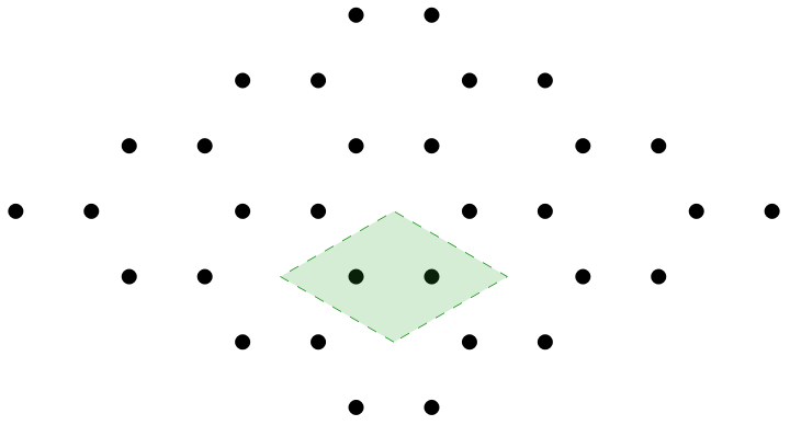
Now lets add some bonds to the lattice. A longitudinal bond is a bond between two balls, possibly in two different unit cells. We specify that syntax as so:
In[]:=
examplespring=
;
2 | {1,0} |
1 | {0,0} |
Meaning “connect ball 2 in Bravais lattice site {1,0} with ball 1 in Bravais lattice site {0,0}”. The order doesn’t matter because this bond is symmetric. There are 3 such bonds in the honeycomb lattice unit cell:
In[]:=
Lsprings=
,
,
;
2 | {1,0} |
1 | {0,0} |
2 | {0,0} |
1 | {0,0} |
2 | {0,0} |
1 | {0,1} |
A torsional bond is a triple of balls, with the bond residing on the middle ball. E.g:
In[]:=
examplespring=
;
1 | {0,0} |
2 | {1,0} |
1 | {1,1} |
Meaning “put a torsional spring between ball 1 in {0,0}, ball 2 in {1,0} and ball 1 in {1,1}. The convention we use is that the bond is centered on ball 2 in {1,0}. There are 6 such bonds in a honeycomb unit cell:
In[]:=
θsprings=
,
,
,
,
,
;
1 | {0,0} |
2 | {1,0} |
1 | {1,1} |
2 | {0,0} |
1 | {0,0} |
2 | {1,0} |
1 | {0,1} |
2 | {0,0} |
1 | {0,0} |
2 | {1,1} |
1 | {0,1} |
2 | {0,0} |
1 | {1,1} |
2 | {1,1} |
1 | {0,1} |
2 | {1,0} |
1 | {1,1} |
2 | {1,1} |
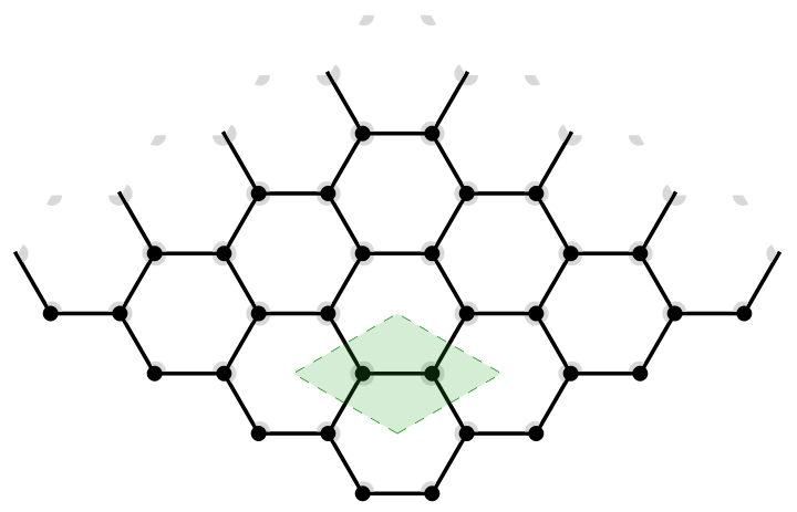
Now lets visualize this lattice. We define keywords, e.g. “torsion, regular” to tell the code what type of bond we are specifying, and what symbol to give its stiffness (“k”, “κ”). We don’t need those symbols yet, but we will do when we compute elastic moduli.
In[]:=
hgeom=bravais,positions,
,Lsprings,k,
,θsprings,κ;hgeomUC=DrawUC[hgeom]hgeomUC=DrawLattice[hgeom]
"extension" |
"regular" |
"torsion" |
"regular" |
Out[]=
Out[]=
Activating the Lattice
Activating the Lattice
The above is a totally passive honeycomb lattice, with linear and torsional rigidity. Our work focuses on active bonds, whose forces and torques break Maxwell-Betti reciprocity [1]. For example, a standard torsional spring has the torque-angle relationship
=-
where the index i is an arbitrary label for some torsional bond i in the unit cell. Our code also implements bonds that act as
τ
i
κδθ
i
where the index i is an arbitrary label for some torsional bond i in the unit cell. Our code also implements bonds that act as
τ
i
a
κ
δθ
i+1
δθ
i-1
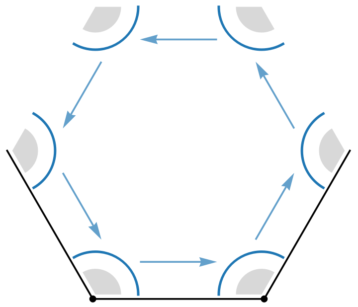
where i+1 and i-1 are labels for neighboring angular bonds. This is explained in great detail in the manuscript [1]! The core idea is that this nearest-neighbor torque-angle relation conserves momentum but does not conserve energy - it “activates” the dynamics of the lattice, creating limit cycle oscillations [3] and non-Hermitian vibrations [1, 2].
In the code, our convention is that these neighbor indices, - i-1, i+1, are specified cyclically. So by including a list as as:
In the code, our convention is that these neighbor indices, - i-1, i+1, are specified cyclically. So by including a list as as:
In[]:=
NRθsprings=
,
,
,
,
,
;
1 | {0,0} |
2 | {1,0} |
1 | {1,1} |
2 | {0,0} |
1 | {0,0} |
2 | {1,0} |
1 | {0,1} |
2 | {0,0} |
1 | {0,0} |
2 | {1,1} |
1 | {0,1} |
2 | {0,0} |
1 | {1,1} |
2 | {1,1} |
1 | {0,1} |
2 | {1,0} |
1 | {1,1} |
2 | {1,1} |
We specify a closed cycle of these non-reciprocal bonds between every torsional bond in the lattice. We visualize this as so:
In[]:=
hgeom=
,
,
,
,1,
,Lsprings,k,
,θsprings,κ,
,NRθsprings,κa;hgeomUC=DrawUC[hgeom]hgeomUC=DrawLattice[hgeom]
1
2
-3 |
3 |
1
2
+3 |
3 |
0 |
0 |
1 |
0 |
"extension" |
"regular" |
"torsion" |
"regular" |
"torsion" |
"data-sharing" |
Out[]=
Out[]=
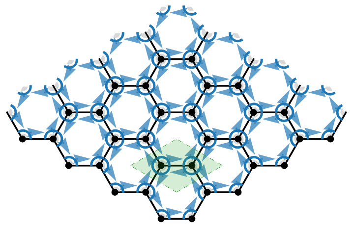
Where the blue arrows indicate who your right and left neighbors are.
Example 2 - Non-reciprocal Longitudinal Bonds
Example 2 - Non-reciprocal Longitudinal Bonds
The manuscript [1] also introduces a non-reciprocal longitudinal bond, with a linear tension-length relation of
Here’s an example using this type of bond in a triangular lattice:
Example 3 - A more complex lattice
Example 3 - A more complex lattice
Here is a more complex lattice - the “Kekule-O” lattice - to put the code through its paces.
Computing Elastic Moduli
Computing Elastic Moduli
So far we have demonstrated code to specify and visualize a lattice. We also implement functions to compute the dynamical matrix - the matrix that encodes the vibrational spectrum - and the elastic moduli of these lattices.
The Vibrational Spectrum
The Vibrational Spectrum
We provide functions that compute analytically the dynamical matrix. I use the triangular lattice from above as an example:
The reciprocal lattice phase factors, q.BravaisVector
Our function to calculate the dynamical matrix
Note that this matrix is non-Hermitian when ka is nonzero. This means that we have a vibrational eigenspectrum featuring gain and loss. Lets sample the Brillouin Zone and plot the eigenspectrum:
We see that the eigenspectrum is indeed complex. The band of modes sitting at small Re[λ] and Im[λ] generate the elastic response of the lattice [1] - the slope of this branch quantifies the so-called “Odd” Modulus.
The Elastic Moduli
The Elastic Moduli
References
References
[1]J. Binysh, G. Baardink, J. Veenstra, C. Coulais & A. Souslov, More is Less in Unpercolated Active Solids. PRX 16 021012 2026.
[2] Scheibner, C. et al. Odd elasticity. Nature Physics 16, 475–480 2020.
[3] J. Veenstra, C. Scheibner, M. Brandenbourger, J. Binysh, A. Souslov, V. Vitelli and C. Coulais, Adaptive Locomotion of Active Solids, Nature 639 935-941 2025.
[4]J. Binysh, J. Veenstra, V. Seinen, R. Naber, D. Robledo-Poisson, A. Hunt, W. van Saarlos, A. Souslov & C. Coulais, Wave Coarsening Drives Time Crystallization in Active Solids. Under Revision in Nature. Preprint: arXiv: 2508.20052.
CITE THIS NOTEBOOK
CITE THIS NOTEBOOK
More is less in unpercolated active solids
by Jack Binysh, Guido Baardink, Jonas Veenstra, Corentin Coulais, and Anton Souslov
Wolfram Community, STAFF PICKS, May 15, 2026
https://community.wolfram.com/groups/-/m/t/3716833
by Jack Binysh, Guido Baardink, Jonas Veenstra, Corentin Coulais, and Anton Souslov
Wolfram Community, STAFF PICKS, May 15, 2026
https://community.wolfram.com/groups/-/m/t/3716833