Abstract
The Wolfram Models have rich and unexplored dynamical properties. In this project we study a class of simple rules (of signatures→ ) that does not change the size of spatial graphs (hypergraphs). Exploring state transition networks shows that, for a phase space of fixed size, by introducing more new elements on the right-side of the rule, the concentrated part of a phase space is decreased, and the transient time required to reach a fixed point is shortened, whose basin of attraction is not necessarily expanding. Moreover, self-loops become increasingly abundant while after a certain point their proportion tends to converge, which could shed light on defining an invariant measure on such evolution systems.
The Wolfram Models have rich and unexplored dynamical properties. In this project we study a class of simple rules (of signatures
n
k
n
k
Typical trajectories for non-growing hypergraph evolutionsFrom a dynamical system point of view, the phase space of a non-growing hypergraph evolution system is a discrete space consisting of all possible hypergraphs of a given signature, and it can be finite or infinite depending on the size of hypergraphs. Given an initial condition, its evolution forms a trajectory. Here are four typical types: after a possible transient stage, it reaches either a fixed point (after which it will not change the appearance but is still evolving), or a limit cycle, or ever-wandering (only for the infinite case), or dead (terminates after finite generations). Some examples are shown in the Table below (the first hypergraph in each row is the initial condition).
In[]:=
Import["table1.png"]
Out[]=
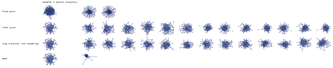
(notes: the first row illustrates a “sunflower” fixed point; the last three rows used the same initial condition; on the second row a 3-cycle is reached after 8 generations; on the third row it has not reached a steady state after 20 generations; the last hypergraph on the last row looks like a creature running away from somewhere.)
State transition networks
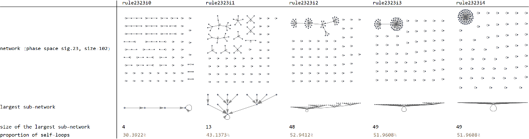
As the evolution does not change the size of a hypergraph, a state transition network can be drawn on the phase space for a given rule. For example, a phase space of signature (sig.23, the first Table below) has 102 nodes representing all 102 inequivalent and connected hypergraphs (two ternary hyperedges). A directed edge connecting two nodes in the network indicates a transition via the rule. Several interesting observations from experiments:
1) a network seems never totally connected. In a finite case, it means that there does not exist a maximal cycle whose length equals to the size of the phase space. Hence no trajectory could possibly visit all places in the phase space;
2) in classification of rules within a signature, for example, signature→ , all the five rules used in the first two Tables below have the same left-side, but introduced 0/1/2/3/4 (rule2323i0/1/2/3/4) new elements on the right-side of the rule. We see that the concentrated part (consisting of sub-networks with more complicated structures than just self-loops) shrinks, and the largest sub-network varies from tree-like to radial-like, implying that average transient time to a fixed point is decreased;
3) analysis on the proportion of self-loops in the network shows that for rules i0 and i1 the proportion increases but interestingly, it seems to stabilise to a fixed value for rules i2, i3 and i4 (~52% for sig.23, and ~26% for sig.33).
State transition networks
As the evolution does not change the size of a hypergraph, a state transition network can be drawn on the phase space for a given rule. For example, a phase space of signature
2
3
2
3
1) a network seems never totally connected. In a finite case, it means that there does not exist a maximal cycle whose length equals to the size of the phase space. Hence no trajectory could possibly visit all places in the phase space;
2) in classification of rules within a signature, for example, signature
2
3
2
3
3) analysis on the proportion of self-loops in the network shows that for rules i0 and i1 the proportion increases but interestingly, it seems to stabilise to a fixed value for rules i2, i3 and i4 (~52% for sig.23, and ~26% for sig.33).
rule2323i0={{1,2,3},{3,4,5}}{{2,3,5},{4,1,3}};rule2323i1={{1,2,3},{3,4,5}}{{2,6,5},{4,1,6}};rule2323i2={{1,2,3},{3,4,5}}{{7,6,5},{4,1,7}};rule2323i3={{1,2,3},{3,4,5}}{{8,6,5},{4,8,7}};rule2323i4={{1,2,3},{3,4,5}}{{9,6,5},{9,8,7}};
Out[]//TableForm=
Out[]//TableForm=
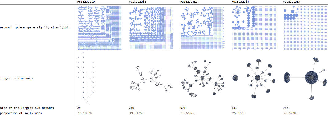
(feel free to magnify any plot)
Another set of examples, where we used a phase space of signature(size = 1,950,935), also shows similar patterns and the largest sub-networks appear even simpler. See Table below.
Another set of examples, where we used a phase space of signature
2
2
3
3
rule2323i0a={{1,2,3},{4,3,2}}{{1,2,4},{3,4,1}};rule2323i1a={{1,2,3},{4,3,2}}{{2,5,3},{5,4,2}};rule2323i2a={{1,2,3},{4,3,2}}{{4,5,6},{6,3,5}};rule2323i3a={{1,2,3},{4,3,2}}{{5,4,7},{4,6,5}};
Out[]//TableForm=
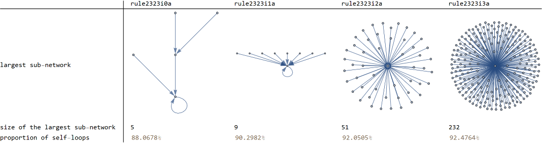
Thoughts on self-loopsReferring to the last Table, where the phase space (size = 1,950,935) is much larger than any previous examples, self-loops can occupy more than 90% of the space, and the largest sub-networks have very simple structures. Self-loop abundance in a large phase space could be a reflection of abundance of isomorphic hypergraphs --- an initial hypergraph (universe) evolves to its first generation after applying the rule, realising it isomorphic to itself, after which it is doomed to repeat itself in later generations, i.e., a self-loop.
2
2
3
3
Notes on ergodicityMy initial motivation was to explore ergodicity in Wolfram Models, as being an important assumption in deriving Einstein’s equations in the models. Direction changed after not finding any trajectory that could visit all places in (or even a large portion of) a phase space. It is still interesting to ask what is the longest possible wandering trajectory or the longest cycle. From the result above, one should look at rules that introduce very few new elements on the right-side. The assumption made in deriving GR in the models is a weak ergodicity on the dynamics of the causal graph. It is yet not clear if any connections can be addressed between ergodic properties on hypergraph evolutions and those on causal graphs. I have read about ergodicity in relativistic settings where one has to choose a reference frame to make sense of a time evolution, and then compare (proper-)time averages with the corresponding ensemble average. Another conceptual difficulty is to identify ensembles in causal graphs.
ConclusionDynamics in state transition networks for non-growing hypergraph evolutions is very rich and worth exploring in detail. By studying some rules with simple signatures we observed interesting behaviour such as non-existence of a maximal cycle, shrinking in the concentrated part, structure change in the largest sub-network, and convergence of the proportion of self-loops. In this short-term project we have only explored an invisible corner of the rulial space as well as all the possible signatures of phase space. To fully understand state transition networks and hence hypergraph evolutions, further research is needed to, for example, classify rules within a signature, explore larger phase spaces, introduce other quantities, etc.
Open questions
Q1: What is the longest trajectory before it reaches a fixed point or a limit cycle or dead, as a function of the rule and size of phase space? For a given rule, does the ratio of the length of the longest wandering trajectory to the size of phase space converge to a fixed value r \in [0, 1]?
Q2: Why, by introducing more new elements on the right-side of the rule, the transient time becomes shorter?
Q3: Why does the proportion of self-loops seem to converge for some rules — is it a general feature or just a coincidence?
Q4: Apart from rules with signatures→ , what are other signatures that can also yield fixed-sized universe?
Q5: How can we define a measure on such phase space, in line with the problem of ergodicity?
...
Q1: What is the longest trajectory before it reaches a fixed point or a limit cycle or dead, as a function of the rule and size of phase space? For a given rule, does the ratio of the length of the longest wandering trajectory to the size of phase space converge to a fixed value r \in [0, 1]?
Q2: Why, by introducing more new elements on the right-side of the rule, the transient time becomes shorter?
Q3: Why does the proportion of self-loops seem to converge for some rules — is it a general feature or just a coincidence?
Q4: Apart from rules with signatures
n
k
n
k
Q5: How can we define a measure on such phase space, in line with the problem of ergodicity?
...
Double bonus
If you manage to read all the way here, please enjoy beauty of nature:
If you manage to read all the way here, please enjoy beauty of nature:
In[]:=
Import["radial1.png"]Import["nature1.png"]
In[]:=
Import["radial0.png"]Import["nature0.png"]
(photo credit : Mile End Park, London, Spring 2020, by Jin)
Appendix
Appendix
Appendix
Metric on phase spaceDefine a metric on a phase space: two hypergraphs , have distance d if one can be transformed to another via at least d steps in the state transition network associated with the rule R: , ) := min{t| = ), i,j = 0, 1, 2, ...}. Consider the minimum distance of order m, , along a trajectory , , , ...} being the minimum distance between and : := , ) = , )). Then for a trajectory reaches i) a fixed point: = 0; ii) a p-cycle: = 0; iiia) a maximal cycle: = 0, where N is the size of a finite phase space; iiib) ever-wandering: ≠ 0 ∀m < ∞, only for an infinite phase space.
H
i
H
j
d(
H
i
H
j
H
j
±t
R
(
H
i
d
m
{
H
0
H
1
H
2
H
i
H
i+m
d
m
min
i⩾0
d(
H
i
H
i+m
min
i⩾0
d(
H
i
m
R
(
H
i
d
1
d
p
d
N
d
m
Rules for experiments
Rules and initial conditions (ic) explored in this project and their typical destinies:
ics: small random hypergraph (10 nodes, ~20 binary edges, and ~5 ternary, 4-ary and 5-ary hyperedges each)
icm1: medium random hypergraph (50 nodes, ~100 binary edges, and ~10 ternary, 4-ary and 5-ary hyperedges each)
icm2: medium random hypergraph (50 nodes, ~600 binary edges, and ~60 ternary, 4-ary and 5-ary hyperedges each)
(i) all 11 rules of signature→ , icm1: after a very short transient, either reaches a fixed point or terminates.
(ii) 45*/178 rules of signature→ , icm2: after a very short transient, reaches either a fixed point or a 2-cycle.
*rule choice: 3 distinct elements on the left-side of the rule, and at least 1 new element on the right-side
(iii) (8+6+7=**) 21/562 rules of signature→ , ics, icm1: after a short transient, reaches either a fixed point, or a p-cycle with small p (observed p = 2, 3), or terminates.
**rule choice: same left-side of the rule, and introducing 0/1/2 new elements on the right-side
(iv) (5+6=***) 11/772,696 rules of signature→ , icm1: either reaches a fixed point, or experiences a long transient, or terminates.
***rule choice: 5 for introducing 0/1/2/3/4 new elements on the right-side of the rule, and 6 for specifying different influences on the new elements
(v) 4/48,554 rules of signature→, icm1: either experiences a long transient, or terminates.
NB: the above results do not represent all possible scenarios, one has to study each state transition network to see the full picture (existence of fixed points, limit cycles of all possible lengths, transient length before termination...).
Rules and initial conditions (ic) explored in this project and their typical destinies:
ics: small random hypergraph (10 nodes, ~20 binary edges, and ~5 ternary, 4-ary and 5-ary hyperedges each)
icm1: medium random hypergraph (50 nodes, ~100 binary edges, and ~10 ternary, 4-ary and 5-ary hyperedges each)
icm2: medium random hypergraph (50 nodes, ~600 binary edges, and ~60 ternary, 4-ary and 5-ary hyperedges each)
(i) all 11 rules of signature
1
2
1
2
(ii) 45*/178 rules of signature
1
3
1
3
*rule choice: 3 distinct elements on the left-side of the rule, and at least 1 new element on the right-side
(iii) (8+6+7=**) 21/562 rules of signature
2
2
2
2
**rule choice: same left-side of the rule, and introducing 0/1/2 new elements on the right-side
(iv) (5+6=***) 11/772,696 rules of signature
2
3
2
3
***rule choice: 5 for introducing 0/1/2/3/4 new elements on the right-side of the rule, and 6 for specifying different influences on the new elements
(v) 4/48,554 rules of signature
3
2
3
2
NB: the above results do not represent all possible scenarios, one has to study each state transition network to see the full picture (existence of fixed points, limit cycles of all possible lengths, transient length before termination...).
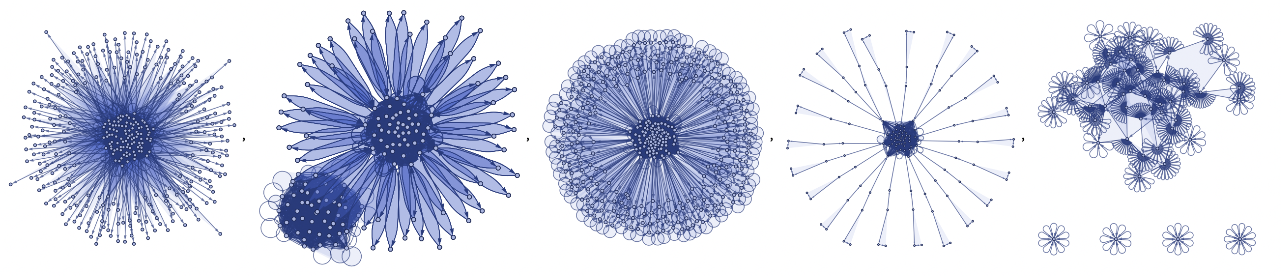
Some artworks
Some artworks
In[]:=
Import["arts.png"]
Out[]=
Keywords
Keywords
◼
Wolfram Models (Wolfram Physics Project)
◼
state transition network
◼
non-growing hypergraph evolution
◼
dynamical systems
◼
ergodicity
Acknowledgment
Acknowledgment
Mentor: Jack Heimrath
Special thanks to Jack, Sam Wilson, Cameron Beetar and József Konczer for helpful discussions, to Jonathan Gorard for great lectures; and to Jesse Friedman for helping running codes on AWS.
Last but not least, thanks Stephen Wolfram for valuable time and inspiring talks.
Last but not least, thanks Stephen Wolfram for valuable time and inspiring talks.
References
References
◼
WPP Sec .3.2 on number of possible rules
◼
WPP Sec .3.3 on number of inequivalent connected initial conditions for small signatures
◼
WPP Sec .3.17 on state networks for systems of limited size and rules without growth
◼
NKS Notes in Sec .6.7 on dynamical systems approaches on cellular automata
◼
◼