Let us consider a sufficiently large constant size of population , and assume that births and
natural deaths are equal . Also newborns and all people of different ages are susceptible.
N
natural deaths are equal . Also newborns and all people of different ages are susceptible.
We assume that each individual of the total population is either susceptible, infectious or recovered from the disease with life - long immunity.
In[]:=

In SIR model, there is no difference between those who are recovered and those who are died; all of them are kept into compartment .
R(t)
In this model, assumes that the population is homogeneous and there is no vital dynamics, that is, the total
population remains constant.
population remains constant.
The highest R0 for the variants Alpha (1.22), Beta (1.19), Gamma (1.21), Delta (1.38) and Omicron (1.90) were reported from Japan, Belgium, the United States, France and South Africa, respectively . Nine out of ten epidemic curves with the highest estimated growth rates and reproduction numbers were due to the Omicron variant indicating the highest transmissibility .[1]
In[]:=
Clear["Global`*"]
In[]:=
betaSoln=First@Solve,β
ℜ
0
β
γ
Out[]=
{βγ}
ℜ
0
In[]:=
params=<|1.90,ββ,γ0.035,10334095,I01|>/.betaSoln
ℜ
0
Out[]=
1.9,βγ,γ0.035,10334095,I01
ℜ
0
ℜ
0
In[]:=
paramsN=Normal@(params//.params)
Out[]=
{1.9,β0.0665,γ0.035,10334095,I01}
ℜ
0
The following rates are based on the paper [2]]
In[]:=
(*infectionRate*)β=0.0665;
In[]:=
(*recoveryrate*)γ=0.035;
In[]:=
(*deathrate*)μ=0.07;
In[]:=
n=1000;
In[]:=
(*FoI*)λ[t_]=βi[t]/n;
In[]:=
tmax=350;
Simple SIR model
Simple SIR model
In[]:=
sireqns1={s'[t]==-λ[t]*s[t],i'[t]==λ[t]*s[t]-γ*i[t],r'[t]==γ*i[t],s[0]==n-20,i[0]==20,r[0]==0};[t]+ℐ[t]+R[t]n;
In[]:=
(*Solvethesystem*)sol1=NDSolve[sireqns1,{s,i,r},{t,0,tmax}];(*Plotthesolutions*)fig1=Plot[Evaluate[{s[t],i[t],r[t]}/.sol1],{t,0,tmax},PlotLegends->{"Susceptible","Infected","Recovered"},AxesLabel->{"Time","Population"},AxesLabel->{"Time","Population"},PlotStyle->{Blue,Red,Green}]
Out[]=
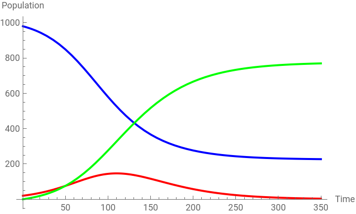


Susceptible : The susceptible refers to a group of people who are not yet infected but may be
infected with the SARS - CoV - 2 virus
infected with the SARS - CoV - 2 virus
Infected : The infected refers to a group of people who have been infected and have infectivity . Infected individuals can spread the disease to susceptible individuals .
Recovered : The removed refers to a group of people who have been removed from the COVID - 19
infected people, such as died, isolated or recovered and are immunized to the SARS - CoV - 2
virus .
infected people, such as died, isolated or recovered and are immunized to the SARS - CoV - 2
virus .
β : infection rate
γ : recovery rate
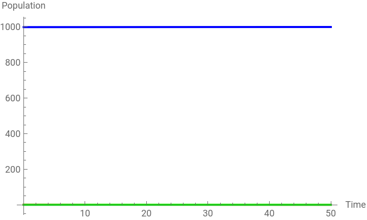
SIR Model with Death and Births
SIR Model with Death and Births
In[]:=
Let the birth rate be , , and death rate . consequently,
b>0
μ>0
bμ
Let the new born babies are quite healthy but susceptible.
In[]:=
b=μ;
In[]:=
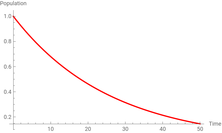
sireqns2={s'[t]==-λ[t]*s[t]-μ*s[t]+b*n,i'[t]==λ[t]*s[t]-γ*i[t]-μ*i[t],r'[t]==γ*i[t]-μ*r[t],s[0]==n-1,i[0]==1,r[0]==0};tmax1=50;
In[]:=
(*Solvethesystem*)sol2=NDSolve[sireqns2,{s,i,r},{t,0,tmax1},MaxStepSize->0.1];(*Plotthesolutions*)fig2=Plot[Evaluate[{s[t],i[t],r[t]}/.sol2],{t,0,tmax1},PlotLegends->{"Susceptible","Infected","Recovered"},AxesLabel->{"Time","Population"},AxesLabel->{"Time","Population"},PlotStyle->{Blue,Red,Green},PlotRange->All]
Out[]=
In[]:=
p2=Plot[Evaluate[{i[t]}/.sol2],{t,0,tmax1},PlotLegends->{"Infected"},AxesLabel->{"Time","Population"},PlotStyle->{Red},PlotRange->All]
Out[]=
Vaccine Efficiency of COVID - 19
Vaccine Efficiency of COVID - 19
Individuals who have taken a full dose of vaccine and they acquire immunity to a particular
infectious disease . A population is said to have herd immunity for COVID - 19 if enough people
are immune so that the disease would not spread .
infectious disease . A population is said to have herd immunity for COVID - 19 if enough people
are immune so that the disease would not spread .
In our model, we consider that our vaccine is 100 % efficiency .
Let is the proportion of the total population is vaccinated and then is the proportion left unvaccinated
p
N
1ï-p
In[]:=
(*vaccinationcoverage*)p=0.2;
In[]:=
sireqns3={s'[t]==-λ[t]*s[t]-μ*s[t]+b*n,i'[t]==λ[t]*s[t]-γ*i[t]-μ*i[t],r'[t]==γ*i[t]-μ*r[t],v'[t]==0,s[0]==(1-p)*n,i[0]==20,r[0]==0,v[0]==p*(n-20)};
In[]:=
(*Solvethesystem*)sol3=NDSolve[sireqns3,{s,i,r,v},{t,0,tmax1}];(*Plotthesolutions*)p3=Plot[Evaluate[{s[t],i[t],r[t],v[t]}/.sol3],{t,0,tmax1},PlotLegends->{"Susceptible","Infected","Recovered","Vaccinated"},AxesLabel->{"Time","Population"},AxesLabel->{"Time","Population"},PlotStyle->{Blue,Red,Green,{Black,Dashed}}]
Leaky vaccine with coverage of 20 %
Leaky vaccine with coverage of 20 %
References
References
1
.Manathunga, S.S., Abeyagunawardena, I.A. & Dharmaratne, S.D. A comparison of transmissibility of SARS-CoV-2 variants of concern. Virol J 20, 59 (2023). https://doi.org/10.1186/s12985-023-02018-x
2
.Mohajan, Haradhan (2022): Mathematical Analysis of SIR Model for COVID-19 Transmission. Published in: Journal of Innovations in Medical Research , Vol. 1, No. 2 (31 August 2022): pp. 1-18. https://mpra.ub.uni-muenchen.de/114390/