The objective of this project to solve a given second order linear partial differential equation with boundary/initial conditions using a convolution neural network. This trained NN estimates the solution of the PDE faster than solving it numerically. This will be a base for a more comprehensive project were a set of NNs will be developed and made ready to solve different categories of PDEs with different boundary/initial condition.
Background
Background
Numerical Solutions to PDEs are time consuming and in some case not available. The idea here is to train a neural network to solve a PDE faster and more efficient compared to existing numerical methods.
This is a continuation of previous work done by Anurag Kamal in 2018. Here, we generalized their work to deliver solutions to any type of second order PDEs with nonlinear boundary/initial conditions
This is a continuation of previous work done by Anurag Kamal in 2018. Here, we generalized their work to deliver solutions to any type of second order PDEs with nonlinear boundary/initial conditions
Methodology
Methodology
Second order linear PDEs are historically categorized into three types: elliptic, parabolic, and hyperbolic. For each category, a neural network chain is constructed. The training data includes density plots of numerical solutions to the given PDE and corresponding numerically-solved solution.
General Form of Second Order PDE
General Form of Second Order PDE
Any second order linear PDE can be written in the following form: A second order linear PDE is called elliptic if . similarly, the PDE is parabolic and hyperbolic if and , respectively.
a[x,y]+2b+c+d+e+fu+g=0
u
xx
u
xy
u
yy
u
x
u
y
Δ=-ac>0
2
b
Δ=0
Δ<0
Nonlinear Boundary Conditions
Nonlinear Boundary Conditions
In this study, the following boundary conditions are used:
where func1 and func2 are nonlinear function including sin, cos, tan, cot, exp, sinh, cosh, tanh.
One choice of func1 are func2 are shown here as examples:
u[x,0]=func1[c1,c2],u[x,1]=0,u[0,y]=func2[c3,c4],u[1,y]=0
where func1 and func2 are nonlinear function including sin, cos, tan, cot, exp, sinh, cosh, tanh.
One choice of func1 are func2 are shown here as examples:
u[x,0]=func1[c1,c2]=c1*
c2*x
e
u[0,y]=func2[c3,c4]=c3*Sinh[c4*x]
Prepare Data for Training the Network
Prepare Data for Training the Network
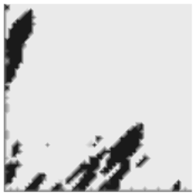
As the first step, each second order linear PDE with desired boundary conditions set is numerically solved for multiple sets of randomly-generated c1, c2, c3, and c4 coefficients. Then, an image of a 10 by 10 constant array for each coefficients is created and then collaged in a single image. This collaged image is served as the input. A density plot of corresponding numerical solution is our desired output.
->

imagesize={120,120};{a,b,c,d,e,f,g} = {1,0,1,0,0,0,0};While[a*c-b^2>=0,{a,b,c,d,e,f,g}=RandomInteger[{0,9},7]]sol[{c1_,c2_,c3_,c4_}]:=NDSolve[a*D[u[x,y],x,x] + 2*b* D[u[x,y],x,y]+ c* D[u[x,y],y,y]+ d* D[u[x,y],x]+ e* D[u[x,y],y]+f*u[x,y]+g==0,u[x,0]0,u[x,1]c1*Exp[c2*x], u[0,y]0,u[1,y]c3*Sinh[ c4*y],u[x,y],{x,0,1},{y,0,1}] Result[{c1_,c2_,c3_,c4_}]:=ColorConvert[DensityPlot[Evaluate[u[x,y]/.sol[{c1,c2,c3,c4}]], {x,0,1},{y,0,1},ColorFunctionScalingFalse,ColorFunctionColorData[{“GrayTones”,{-0.05,0.05}}], PlotLegendsFalse,BoundaryStyleNone,FrameFalse],GrayLevel] rawElliptic[{c1_,c2_,c3_,c4_}]:=ImageCollage[ Image[ConstantArray[(c1/50), {10,10}]], Image[ConstantArray[(c2/50), {10,10}]], Image[ConstantArray[(c3/50), {10,10}]], Image[ConstantArray[(c4/50), {10,10}]]] c1Set = c1Set = RandomReal[{0.1,10},{10,4}];datatotal = rawElliptic[#] -> Result [#]& /@c1Set ;
Neural Network Structure
Neural Network Structure
A. Hyperbolic Second Order Linear PDE
A. Hyperbolic Second Order Linear PDE
The neural network developed for hyperbolic PDEs has the following structure:
NetChain


ResultsHyperbolic PDEs can be estimated using the designed NN. There is a 85% probabiity that the error of this estimation is less than 10%. The error histogram on 500 instances is shown below.
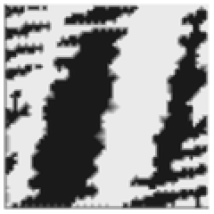
And here you can see an example of the NDSolve and NN estimations:
And here you can see an example of the NDSolve and NN estimations:
,

,
,
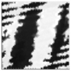
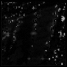
First image is the raw image which is a collage of constant arrays of four parameters c1 to c4. The second image is the result of solving the PDE and given boundary conditions using NDSolve. The estimation of NN is shown is third image. Finally, the last image is the difference between estimations by NDsolve and NN.