Introduction
Introduction
Stock market returns have been shown to have power tails for the extremes of their distributions, with a tail exponent, α, having a value near 3. Yet when the inputs to continuous double auction [CDA] market systems have been studied, the implied returns from the buy and sell order books have heavy power tailed distributions in the domain of attraction of Stable distributions. But the output returns of market prices have power tails which are lighter than the Stable distribution domain of attraction. This suggests that the CDA may be acting like a filtering mechanism in the process of matching buy and sell orders to make a transaction. Suppose that half of the most extreme orders of the buy and sell orders never match, but the power tail structure of the order books still drives trading. In this case rather than having return outputs like a Stable distribution, the output might look like the middle of three Stable order statistic distributions. Suppose the CDA black box puts out a set of logarithmic returns that looks like the middle of three random variables from a Stable distribution, then the return distribution might be modeled by a Stable 2:3 order statistic distribution. The rest of this notebook presents this distribution and demonstrates algorithms that can use the Stable 2:3 order distribution to model financial returns.
Stable 2:3 order statistic distribution
Stable 2:3 order statistic distribution
The S23OrderDistribution is defined similarly to the Mathematica StableDistribution with four parameters, {α, β, μ, σ} and two types, {0, 1}. The α parameter has been changed to be double the StableDistribution, with a range for α of (0, 4], so that it gives the tail exponent of S23OrderDistribution. The algorithms in the package will not work below α = 0.5. For calculations in the algorithms α /2 is passed to the built-in StableDistribution.
α Shape parameter and distribution tail exponent (0, 4]β Skewness parameter [-1, 1]μ Location parameter [μ ∈ Reals]σ Scale parameter [σ > 0]
The fitting is done in the type = 0 because it is continuous as α approaches 1. But the calculations in this notebook for financial data will be in type = 1, because μ, carries some information about the mean of the return data.
In[]:=
Needs["S23OrderDistribution`"]
In[]:=
?S23OrderDistribution
Out[]=
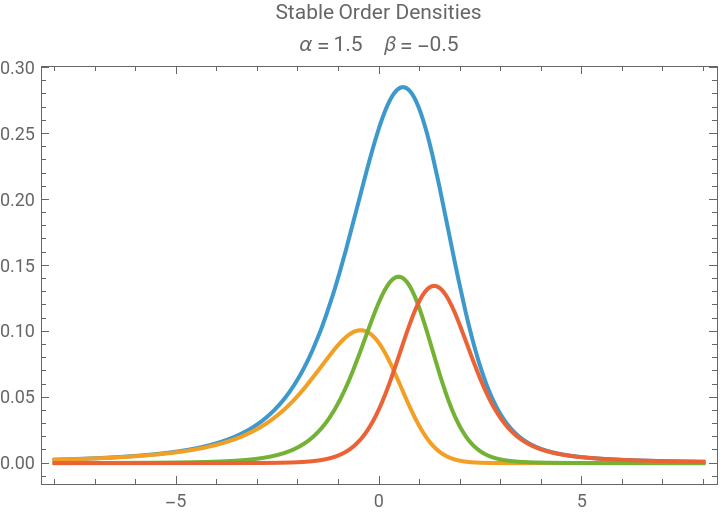
The graph below shows the parent StableDistribution in blue and the three order distributions scaled by 1/3. The average of the three order statistic PDFs will equal the parent distribution PDF.
{alpha,beta}={1.5,-0.5};sd=StableDistribution[alpha,beta];plot1=PlotTooltip[PDF[OrderDistribution[{sd,1},1],x]," Density"],TooltipPDF[OrderDistribution[{sd,3},1],x]3," Density",TooltipPDF[OrderDistribution[{sd,3},2],x]3," Density",TooltipPDF[OrderDistribution[{sd,3},3],x]3," Density",{x,-8,8},
X
1:1
X
1:3
1
3
X
2:3
1
3
X
3:3
1
3
Out[]=
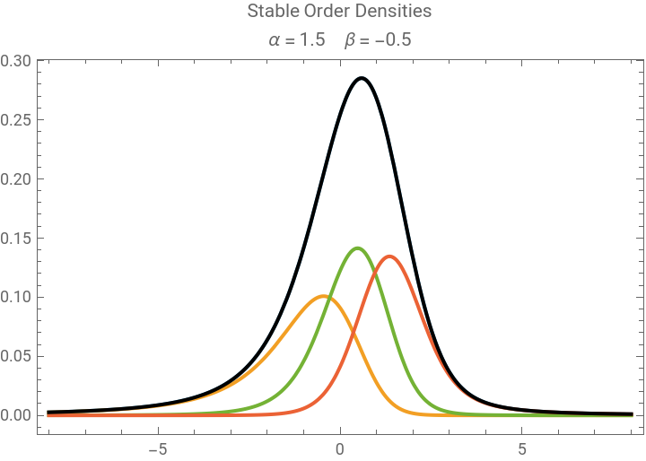
The plot below demonstrates that the mean of the three distributions in black matches the parent distribution above in blue.
Showplot1,PlotMean[{PDF[OrderDistribution[{sd,3},1],x],PDF[OrderDistribution[{sd,3},2],x],PDF[OrderDistribution[{sd,3},3],x]}],{x,-8,8},
Out[]=
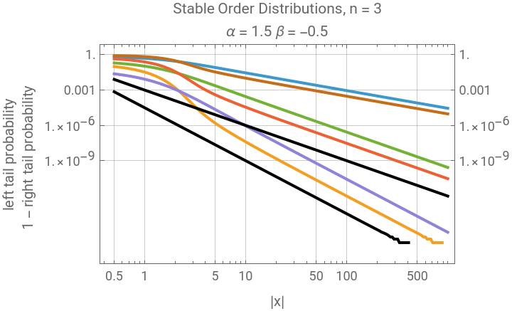
This plot demonstrates the tail behavior for each of the ranks of a set of 3rd order Stable Distributions, which have their slopes shown on a LogLogPlot in colors. The black lines demonstrate ParetoDistribution with 2 α and 3 α slopes for comparison.
The right tail of the 1:3 and the left tail of the 3:3 are on top with a tail exponent of 3 α, the lightest tail. The left 1:3 til and the right 3:3 tails are the colored tails near the bottom with the heaviest tail exponent of 1α. The 2:3 tails are in the middle and both have the tail exponent of 2 α.
The right tail of the 1:3 and the left tail of the 3:3 are on top with a tail exponent of 3 α, the lightest tail. The left 1:3 til and the right 3:3 tails are the colored tails near the bottom with the heaviest tail exponent of 1α. The 2:3 tails are in the middle and both have the tail exponent of 2 α.
{alpha,beta}={1.5,-0.5};max=10^3;sd=StableDistribution[alpha,beta];LogLogPlot{CDF[OrderDistribution[{sd,3},1],-x],1-CDF[OrderDistribution[{sd,3},1],x],CDF[OrderDistribution[{sd,3},2],-x],1-CDF[OrderDistribution[{sd,3},2],x],CDF[OrderDistribution[{sd,3},3],-x],1-CDF[OrderDistribution[{sd,3},3],x],1-CDF[ParetoDistribution[0.1,2alpha],x],1-CDF[ParetoDistribution[0.1,3alpha],x]},{x,0.5,max},
Out[]=


Fitting stock market returns
Fitting stock market returns
The algorithm below generates a report for a stock market ticker symbol using FinancialData. It takes as inputs the ticker symbol as a string and the startDate as DateObject. To show the tail effects of the S23OrderDistribution generally requires a sample size of 500 or more, A start date of at least two years ago will have about 500 points, Larger samples will increase function time as fitting and drawing the PDF are relatively slow. This function is used in the notebook supplement to demonstrate the quality of fits for a large sample of stocks.
Clear[S23FitReport];lr=0;S23FitReport[tickerSymbol_String,startDate_DateObject]:=Module{data,(*lr,*)pLevel,lrQrng,lrD,parm0,skd,dt,α,β,μ,σ,s23d,HTs23d},data=FinancialData[tickerSymbol,startDate,Method->"Legacy"];Print[DateListPlot[data,PlotRangeAll,JoinedTrue,GridLines->Automatic,PlotLabeltickerSymbol<>" Closing Price"]];(*Print[DateListLogPlot[data,PlotRangeAll,JoinedTrue,PlotLabeltickerSymbol<>" Closing Price\nLog Scale"]];*)lr=Differences[Log[data[[All,2]]]];dt=Rest[data[[All,1]]];pLevel=0.02;lrQrng=Quantile[lr,{pLevel,1-pLevel}];Print[DateListPlot[Tooltip@{Transpose[{dt,lr}],Select[Transpose[{dt,lr}],!lrQrng[[1]]<#[[2]]<lrQrng[[2]]&]},PlotStyle{{StandardBlue,PointSize[0.01]},{StandardRed,PointSize[0.01]}},PlotRangeAll,Joined->False,GridLines->Automatic,PlotLabeltickerSymbol<>" Daily Log Returns\np = "<>ToString[pLevel,TraditionalForm]<>" Extremes Red"]];lrD=EmpiricalDistribution[lr];s23d=EstimatedDistribution[lr,S23OrderDistribution[α,β,μ,σ]];parm0=List@@s23d;Print[tickerSymbol," Stable 2:3 Order Statistic Distribution Parameters, {α, β, μ, σ, type}:\n",parm0,"\nDistribution Fit Test"];HTs23d=DistributionFitTest[lr,s23d,"HypothesisTestData"];Print[HTs23d["TestDataTable",All],"\n"];PrintLogLogPlot{CDF[lrD,-x],1-CDF[lrD,x],CDF[s23d,-x],1-CDF[s23d,x]},{x,0.001,Max[Abs[lr]]5/4},;skd=SmoothKernelDistribution[lr];Print[Plot[{PDF[s23d,x],PDF[skd,x]},{x,Min[lr],Max[lr]},PlotRangeAll,PerformanceGoal"Speed",PlotLabeltickerSymbol<>" PDF - Blue\nEmpirical PDF - Yellow"]];(*Print[LogLogPlot[{PDF[S23OrderDistribution[parm0],-x],PDF[S23OrderDistribution[parm0],x],PDF[skd,-x],PDF[skd,x]},{x,0.005,Max[Abs[lr]]},PlotRangeAll,PerformanceGoal"Speed",PlotLabel"LogLogPDF Tail Fits"]];*)Print["*****End "<>tickerSymbol<>" Report*****\n"];;
In[]:=
startDate=DatePlus[Today,{-2,"Year"}]S23FitReport["CME",startDate]
Out[]=
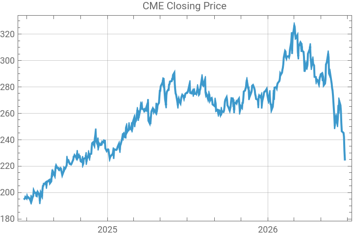
The first graphic above shows the daily closing price plot for the stock.
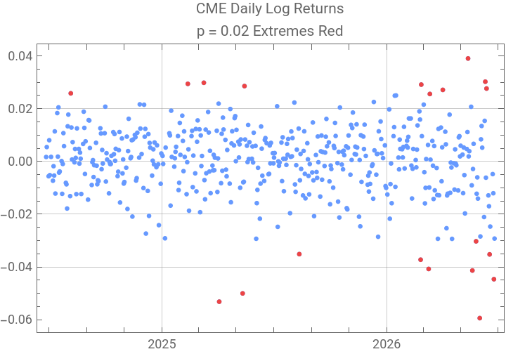
The next plot shows all the points of log returns for the two year price data. The red points are in the lower and upper 0.02 quantiles of the data. It is important to note that high magnitudes of both positive and negative returns tend to cluster in financial data. This means the magnitudes of market returns are serially dependent so that although the distribution fit to the data may be excellent, there is limited ability to use the distribution to predict future returns with statistical methods which assume independent random variables.
The next panel shows the results of the fit, the tail exponent, α, is close to 3; β is significantly negatively skewed. Then is the result of DistributionFitTest which shows remarkably good p-values for the fit using a variety of methods.
The tail fitting is shown with a LogLogPlot of the right and left tails. The right tails are in red. The EmpericalDistribution from the data have irregular steps, because 1/sampleSize is not a particularly good estimate for the probability of a heavy tailed event. The distribution fit curve is smooth and deliberately extended beyond the data to help show the linearity of the function in a LogLogPlot. In this case there are not really any right tail events in the data.
The last graph in the report shows a comparison to the S23OrderDistribution PDF, in blue to empirical SmoothKernelDistribution PDF in yellow. The graph demonstrates the accuracy of the fit to the central part of the distribution and nicely shows the skewness.
The expectation of the distribution can be estimated by NIntegrate.
Variance may also be checked.
There likely a closed formula for the mean from the parameters, but I do not yet know f(α). At β = 0, the distribution is symmetric and the mean = μ.
Summary
Summary
I presented this distribution 13 years ago in this forum. Since then computers and Mathematica have become much faster, making the algorithms more useable. There are more built-in functions like DistributionFitTest. The distribution fits to daily log return data have also stood the test of time, especially as high frequency trading strategies have become more sophisticated and prevalent. If anything the fits today are better.
When I posted this 13 years ago there was some discussion that it was unnecessary because EmpiricalDistributions could be used instead, but this is not true if you are interested in tail events or how the CDA market actually behaves statistically. Take a look at a large number of fits in the notebook supplement. Such accurate fitting suggests that the S23OrderDistribution may actually tell us something about the stochastic processes in the CDA. The model assumes that Ask and Bid orders may be symmetric, the generalized central limit theorem for heavy tails is alive and well inside the CDA. If the model is a true model for the CDA, then it probably provides an accurate estimate for α, which could be used for assessment of the magnitude of risk related to market crashes.
When I posted this 13 years ago there was some discussion that it was unnecessary because EmpiricalDistributions could be used instead, but this is not true if you are interested in tail events or how the CDA market actually behaves statistically. Take a look at a large number of fits in the notebook supplement. Such accurate fitting suggests that the S23OrderDistribution may actually tell us something about the stochastic processes in the CDA. The model assumes that Ask and Bid orders may be symmetric, the generalized central limit theorem for heavy tails is alive and well inside the CDA. If the model is a true model for the CDA, then it probably provides an accurate estimate for α, which could be used for assessment of the magnitude of risk related to market crashes.
References
References
1. Zovko I., Farmer J. D. 2002 The power of patience: a behavioral regularity in limit order placement Quantitative Finance 2 387
2. Potters M., Bouchaud J.P. 2003 Statistical properties of stock order books: empirical results and models Physica A 324 133
3. Smith, E., Farmer, J.D., Gillemot, L., Krishnamurthy, S., Statistical theory of the continuous double auction, Quantitative Finance, 3, 481-514.
CITE THIS NOTEBOOK
CITE THIS NOTEBOOK
Stable 2:3 order statistic distribution for stock market returns
by Robert Rimmer
Wolfram Community, STAFF PICKS, June 27, 2026
https://community.wolfram.com/groups/-/m/t/3739392
by Robert Rimmer
Wolfram Community, STAFF PICKS, June 27, 2026
https://community.wolfram.com/groups/-/m/t/3739392