This computational essay is a continuation of my previous work on standard quantum adiabatic evolution, now extending it to the local adiabatic framework introduced by Jérémie Roland and Nicolas J. Cerf. In this project, I explore how enforcing the adiabatic condition locally in time allows us to recover the quadratic speedup of Grover’s search algorithm. In contrast, the standard linear interpolation schedule is shown to yield only classical O(N) scaling.
Quantum Search Problem: Two-Qubit Adiabatic Search Example
Quantum Search Problem: Two-Qubit Adiabatic Search Example
Adiabatic Evolution
Adiabatic Evolution
Quantum computation can be formulated not only in terms of discrete gate-based circuits, but also as a continuous-time dynamical process governed by a time-dependent Hamiltonian. Within this paradigm, the adiabatic theorem provides a powerful framework: if a quantum system is evolved slowly enough, it remains close to its instantaneous ground state, allowing one to encode the solution of a computational problem in the final Hamiltonian.
More precisely, consider a system evolving under a Hamiltonian , with instantaneous eigenstates and eigenvalues (t).
H(t)
|(t)〉
E
k
E
k
A quantitative version of this statement is given by the adiabatic condition:
〈(t)||(t)〉
E
1
H
t
E
0
2
g(t)
where is the instantaneous spectral gap and controls the allowed error.
g(t)=(t)-(t)
E
1
E
0
ϵ≪1
The adiabatic framework becomes particularly relevant in the context of quantum search algorithms. By designing a time-dependent Hamiltonian whose final ground state corresponds to the marked element, the search task can be reformulated as an adiabatic evolution problem. The runtime is then determined by the spectral properties of the interpolating Hamiltonian, especially the minimum gap appearing in the adiabatic condition. This establishes the unstructured search problem as a paradigmatic example of adiabatic quantum computation.
Search Problem Setup
Search Problem Setup
We begin by considering the unstructured search problem, originally introduced by Lov Grover. Given a set of N items, one of which is marked, the goal is to identify the marked element using as few queries as possible. Classically, this requires evaluations.
(N)
In the adiabatic setting, we encode the problem using n qubits, so that the Hilbert space has dimension . The computational basis states represent the database elements, and the marked item corresponds to an unknown state that we aim to reach through the evolution.
N=
n
2
N-1
{|i〉}
i=0
|m〉
Before diving in, we set up our computational environment by loading the Wolfram Quantum Framework alongside the Quantum Optimization Paclet:
In[]:=
<<Wolfram`QuantumFramework`<<Wolfram`QuantumFramework`QuantumOptimization`
We start from the uniform superposition:
|〉=|i〉
ψ
0
1
N
N-1
∑
i=0
To make things concrete, we begin with a simple example of qubits (). We initialize the system in the uniform superposition over all basis states:
n=2
N=4
In[]:=
ψ0=QuantumState["UniformSuperposition"[2]]
Out[]=
1
2
1
2
1
2
1
2
which assigns equal probability amplitude to every possible solution.
The computational basis states are:
In[]:=
ψ0["BasisStates"]
Out[]=
{,,,}
|00〉
|01〉
|10〉
|11〉
representing the four elements of the database.
To drive the system from the initial state to the solution, for this example we first define the marked state as:
|ψ〉
|m〉
In[]:=
m=QuantumState["Register"[2,2]]
Out[]=
|10〉
which represents the item we are searching for. In the computational basis, this corresponds to one of the basis vectors { , but its identity is unknown a priori.
N-1
{|i〉}
i=0
Hamiltonian Construction
Hamiltonian Construction
We now construct two Hamiltonians whose ground states encode the initial and target configurations.
The initial Hamiltonian is defined as
H
0
ψ
0
ψ
0
In[]:=
h0=QuantumOperator["II"]-ψ0["Operator"]
Out[]=
3
4
1
4
1
4
1
4
1
4
3
4
1
4
1
4
1
4
1
4
3
4
1
4
1
4
-|11〉〈01|-|11〉〈10|+|11〉〈11|
1
4
1
4
3
4
so that its ground state is the uniform superposition. The problem Hamiltonian is:
H
m
In[]:=
hm=QuantumOperator["II"]-m["Operator"]
Out[]=
|00〉〈00|+|01〉〈01|+|11〉〈11|
whose ground state is precisely the marked state.
The system evolves under the searching (interpolating) Hamiltonian , where :
H(s)=(1-s)+s
H
0
H
m
s=t/Tands∈[0,1]
In[]:=
h=(1-s)*h0+s*hm
Out[]=
3(1-s)
4
1
4
1
4
1
4
1
4
3(1-s)
4
1
4
1
4
1〉〈11|+(-1+s)|10〉〈00|+(-1+s)|10〉〈01|+|10〉〈10|+(-1+s)|10〉〈11|+(-1+s)|11〉〈00|+(-1+s)|11〉〈01|+(-1+s)|11〉〈10|+
1
4
1
4
3(1-s)
4
1
4
1
4
1
4
1
4
3(1-s)
4
+s|11〉〈11|
System Instantaneous Eigenvectors
System Instantaneous Eigenvectors
We now compute the instantaneous eigenvectors of the interpolating Hamiltonian and simulate the adiabatic evolution of the system in order to analyze how the ground state continuously transforms into the marked state throughout the evolution:
In[]:=
evolution=QuantumAdiabaticEvolve[h0,hm,"Parameter"->s]
Out[]=
QuantumAdiabaticEvolution

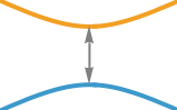
The adiabatic evolution is simulated using the QuantumAdiabaticEvolve function. Further details and documentation can be found here.
Using QuantumAdiabaticEvolve, we compute the instantaneous eigenvalues and eigenvectors of the interpolating Hamiltonian and analyze the resulting adiabatic evolution:
In[]:=
evolution["Energies"]
Out[]=
1-1+
1
2
1-3s+3
,2
s
1
2
1-3s+3
,1,12
s
In[]:=
evolution["LowestEnergyEigenvector"]
Out[]=
1
2
3-3s+1
+12
s
2
3-3s+1
-2s+12
s
1
2
3-3s+1
+12
s
2
3-3s+1
-2s+12
s
3-3s+1
+12
s
+3
3-3s+1
-2s+12
s
2
3-3s+1
+12
s
2
3-3s+1
-2s+12
s
1
2
3-3s+1
+12
s
2
3-3s+1
-2s+12
s
In[]:=
evolution[{"EnergySpectrumPlot","AdiabaticPathPlot"}]
Out[]=
,
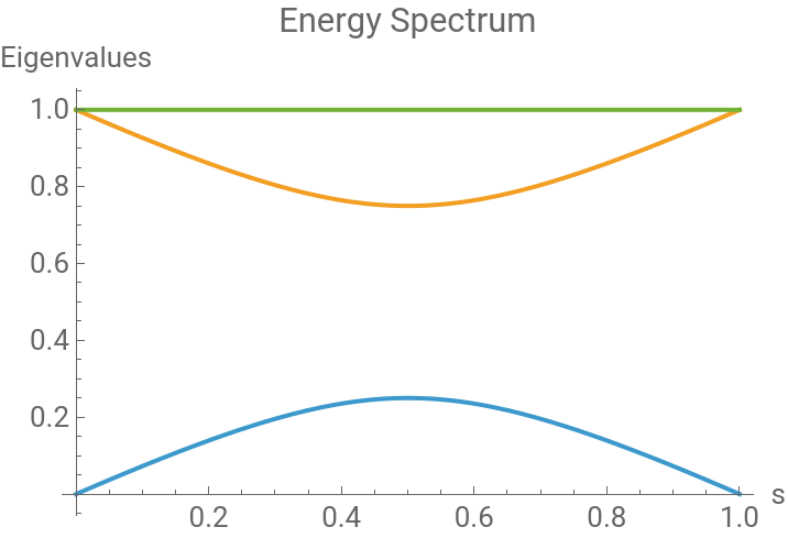


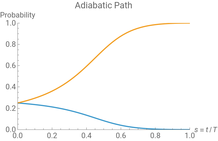
Although adiabatic quantum search is often associated with Grover-like quadratic speedup, this advantage is not automatically obtained for arbitrary interpolation schedules. In particular, using the standard linear schedule causes the runtime of the search Hamiltonian to scale as , eliminating the quantum advantage. The purpose of the following section is to explicitly derive this limitation and motivate the need for the local adiabatic schedule introduced later.
s=t/T
(N)
Scaling of Standard Adiabatic Search
Scaling of Standard Adiabatic Search
While the two-qubit example illustrates the mechanics of adiabatic search, understanding its computational efficiency requires analyzing the general N-dimensional case. We therefore now study how the spectral gap scales with system size and how this affects the runtime of the standard adiabatic evolution.
For further analysis, we now compute the energy gap for the search Hamiltonian and extend the construction to a general system of qubits. We begin by evaluating the gap numerically for small systems, increasing the number of qubits from up to .
n
n=2
n=6
In standard adiabatic algorithms, one introduces an interpolation parameter and defines:
s(t)∈[0,1]
H(t)=H(s(t))=(1-s)+s
H
0
H
m
In[]:=
H0=Table[QuantumOperator["I",n]-QuantumState["UniformSuperposition"[n]]["Operator"],{n,2,6}];
In[]:=
Hm=Table[QuantumOperator["I",n]-QuantumState["Register"[n,2]]["Operator"],{n,2,6}];
We then construct the searching Hamiltonian for each system size:
H(s)
In[]:=
H=MapThread[QuantumAdiabaticEvolve[#1,#2,"Parameter"->s]&,{H0,Hm}];
For each case, we compute the spectral gap as the difference between the two lowest eigenvalues:
In[]:=
energyGaps=FullSimplify[Through[H["EnergyGap"]],0<=s<=1]
Out[]=
,,
1+3(-1+s)s
,2+7(-1+s)s
2
1
2
4+15(-1+s)s
,8+31(-1+s)s
2
2
1
4
16+63(-1+s)s
We observe a clear pattern in the dependence on s as the system size increases. To extract a general expression, we look at the coefficient of in :
s(s−1)
2
g(s)
In[]:=
seq=FindSequenceFunctionCoefficient[#,s(s-1)]&/@,n
2
energyGaps
Out[]=
1-n
2
1+n
2
Calculating the minimal gap for each case:
We determine the minimal gap in function of N:
Using the chain rule, we can rewrite the time derivative of the Hamiltonian as:
Substituting this into the adiabatic condition:
We find the following bound:
From the resulting plots, we observe that the transition matrix element remains strictly below 1 throughout the entire evolution interval:
This observation is one of the central insights of adiabatic quantum search and directly motivates the local adiabatic strategy proposed by Roland and Cerf, where the evolution rate is continuously adapted to the instantaneous gap.
Local Adiabatic Evolution
Local Adiabatic Evolution
The key observation is that the adiabatic condition is local in time: the allowed evolution rate depends on the instantaneous spectral gap. Since the gap becomes exponentially smaller only in a narrow region around the avoided crossing, the evolution should slow down only there rather than throughout the entire computation.
Following Roland and Cerf, we therefore impose the adiabatic condition locally by choosing the evolution rate to saturate the bound:
Using the analytical expression previously derived for the gap, we can directly integrate the differential equation governing the schedule.This yields the closed-form expression for the evolution time:
References
References
◼
Jérémie Roland and Nicolas J. Cerf. Quantum Search by Local Adiabatic Evolution. Physical Review A 65, 042308 (2002). https://journals.aps.org/pra/abstract/10.1103/PhysRevA.65.042308.
◼
W. van Dam, M. Mosca and U. Vazirani. How powerful is adiabatic quantum computation?. Proceedings 42nd IEEE Symposium on Foundations of Computer Science. https://ieeexplore.ieee.org/document/959902
◼
Tameem Albash and Daniel A. Lidar. Adiabatic Quantum Computation. Rev. Mod. Phys. 90, 015002 (2018). https://journals.aps.org/rmp/abstract/10.1103/RevModPhys.90.015002.
◼
Avik Mitra, Arindam Ghosh, Ranabir Das, Apoorva Patel, and Anil Kumar. Experimental Implementation of Local Adiabatic Evolution Algorithms by an NMR Quantum Information Processor. Journal of Magnetic Resonance 177, 285–298 (2005). https://www.sciencedirect.com/science/article/abs/pii/S1090780705002776
CITE THIS NOTEBOOK
CITE THIS NOTEBOOK
Symbolic local adiabatic quantum search: spectral analysis, complexity scaling, and quantum speedup
by Sebastian Rodriguez
Wolfram Community, STAFF PICKS, June 9, 2026
https://community.wolfram.com/groups/-/m/t/3730715
by Sebastian Rodriguez
Wolfram Community, STAFF PICKS, June 9, 2026
https://community.wolfram.com/groups/-/m/t/3730715