Cellular Automata with Global Control are cellular automata (CA), whose rules depend on global features of their recent state. An example of this type of CA is that two of the 256 elementary CA are combined and the rule applied at each step depends on whether the number of black cells is even or odd. Other possible types of global control depend on the fraction of black cells and the rule applied at each step depends on whether the fraction of black cells is greater than a given threshold.
Since there are 65536 different possible CA with global control for every single type of coupling (and every single choice of parameters affecting the coupling), automated analysis of the resulting behaviour is necessary in order to make an exhaustive analysis of these systems possible. We study some statistical properties of these kind of CA.
Some Criteria for Classifying CA with Global Control
Some Criteria for Classifying CA with Global Control
According to Stephen Wolfram’s original classification there are 4 classes which distinguish CA. Class 1 contains all CA whose evaluation lead to a fixed point, independent of their initial condition. Class 2 contains all CA which become periodic. Class 3 CA appear chaotic and random. The main feature of class 4 CA are localized structures, which interact in a complicated way - these automata are neither completely random nor ordered. We will try to establish similar classes for globally controlled CA.
To implement a globally controlled CA, our function creates a list of the states at each step and, (as a single number) the background:
In[]:=
GCCA[{r1_,r2_},{init_,bg_},t_]:=
The function stops the evaluation when the cellular automaton “died out”, i.e. only the background pattern remains. Therefore, class 1 behaviour is already detected during evaluation.
To analyze the periodic behaviour, the function FindTransientRepeat was applied to single diagonals and columns. So we need three functions which are directly applied to the lists returned by GCCA and return the the periodic behaviour as well as the transient phase before:
In[]:=
LeftDiagonalPeriodicyCheck[tca_,column_]:=LeftDiagonalPeriodicyCheck[tca,column,2];LeftDiagonalPeriodicyCheck[tca_,column_,repeats_]:=FindTransientRepeat[Join[tca[[1;;Floor[column/2],2]],tca[[(1+Floor[column/2]);;-1,1,column]]],repeats];RightDiagonalPeriodicyCheck[tca_,column_]:=RightDiagonalPeriodicyCheck[tca,column,2];RightDiagonalPeriodicyCheck[tca_,column_,repeats_]:=FindTransientRepeat[Join[tca[[1;;Floor[column/2],2]],tca[[(1+Floor[column/2]);;-1,1,-column]]],repeats];ColumnPeriodicyCheck[tca_,column_]:=ColumnPeriodicyCheck[tca,column,2];ColumnPeriodicyCheck[tca_,column_,repeats_]:=FindTransientRepeat[Join[tca[[1;;Abs[column],2]],Extract[tca[[1+Abs[column];;Length[tca],1]],Array[{#,If[column>0,2column+#,#]}&,Length[tca]-Abs[column]]]],repeats];
The idea was to characterize the classes of behaviour by analyzing many columns and diagonals of the global controlled CA and compare this with the behaviour of the elementary CA. Indeed, periodic behavior as well as nested patterns can often be detected by this analysis. Unfortunately, there are exceptions. Even elementary CA rule 30, for example shows a lot periodic behaviour on the left hand side and also the diagonals on the right hand side are all periodic (although with rapidly increasing periods, therefore it cannot be properly detected if too few steps are evaluated). Non periodic behaviour (i.e. “chaos”) will only be detected when analysing the columns. Things become even more complicated when growth becomes irregular as it often happens on global controlled CA due to rule change. For simplicity, the following show only the lengths of transients and repeats. This example shows how the lengths of periods (if they exist) depend on which diagonal slice through the CA we consider. Consider for example the rule GCCA where rule 30 is coupled with itself:
In[]:=
data30=GCCA[{30,30},{{1},0},750];Manipulate[Panel[Style[Column[{Row[{"left:",Map[Length,LeftDiagonalPeriodicyCheck[data30,l],{1}]}],Row[{"column:",Map[Length,ColumnPeriodicyCheck[data30,col],{1}]}],Row[{"right:",Map[Length,RightDiagonalPeriodicyCheck[data30,r],{1}]}]}],12]],{l,1,50,1},{col,-50,50,1},{r,1,50,1},LabelStyle->Directive[12],SaveDefinitionsTrue]
Out[]=


This particular global controlled CA shows chaotic behaviour until it suddenly turn into repetitive behaviour (while shifting the the right) after 558 steps. Nevertheless, there are left diagonals and columns, where that cannot be properly detected. The reason is that these diagonals and columns hit the remaining structure after step 558.
In[]:=
data=GCCA[{11,28},{{1},0},750];Manipulate[Panel[Style[Column[{Row[{"left:",Map[Length,LeftDiagonalPeriodicyCheck[data,l],{1}]}],Row[{"column:",Map[Length,ColumnPeriodicyCheck[data,col],{1}]}],Row[{"right:",Map[Length,RightDiagonalPeriodicyCheck[data,r],{1}]}]}],12]],{l,1,1000,1},{col,-50,750,1},{r,1,50,1},LabelStyle->Directive[12],SaveDefinitionsTrue]
Out[]=
In[]:=
Image[1-RectangularGCCA[data]]
Out[]=
Another Try to Classify the Global Controlled CA
Another Try to Classify the Global Controlled CA
Another idea was to analyse the structures within the evaluation of the elementary CA and compare them with the structures which arise in global controlled CA. There are two possibilities, how to compare structures:
1) exact comparison, i.e within the pattern all white cells must be white and all black cells must be black in both automata.
2) look, if some white area in the elementary CA “fit into” a white area of the global controlled CA, i.e. a black cell in the pattern is allowed to be white in the global controlled CA but all white cells must be white in both automata.
Statistics on Global Controlled CA with Random Initial Conditions
Statistics on Global Controlled CA with Random Initial Conditions
(Tests with Global Controlled CA whose Rule Depends on the Fraction of Black Cells)
In[]:=
GCCAMajority[{r1_,r2_},{init_,bg_},threshold_,t_]:=NestWhileList[{GCCAMajoritystep[{r1,r2},First[#],Last[#],threshold],CellularAutomaton[{r1,r2}[[If[Mean[CleanCA[First[#],Last[#]]]<threshold,1,2]]],ConstantArray[#[[2]],3],1][[-1,2]]}&,{init,bg},MemberQ[#[[1]],1-#[[2]]]&,1,t]
In[]:=
GCCAMajoritystep[{r1_,r2_},init_,bg_,threshold_]:=CellularAutomaton[{r1,r2}[[If[Mean[CleanCA[init,bg]]<threshold,1,2]]],Join[{bg},init,{bg}],{1,All}][[-1]]
We compare how some statistical measures behave, if we run the global controlled CA with
1) one randomly chosen Initial conditions,
2) 5 randomly chosen Initial conditions (considering the mean value of corresponding cells),
3) 50 randomly chosen Initial conditions (considering the mean value of corresponding cells). In this last case, it is also shown, how these statistical measures stabilizes, if one increases the number of steps.
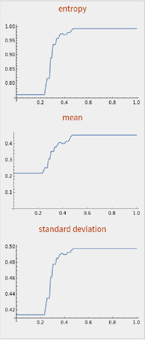
For each set of automata we compute the base 2 information entropy, mean of all values of the cellular automata and the standard deviation over all cells. The x-axis shows the proportion of black cells required to change the rule which is applied.
The following code can also guess the statistical distribution of the automaton’s cells.
One Initial Condition
One Initial Condition
Out[]=
Five Different Initial Conditions
Five Different Initial Conditions
Fifty Different Initial Conditions
Fifty Different Initial Conditions
Determine the effect of the number of calculated rows on the statistical measures:
Again, another visualisation showing different possible rule combinations and generated mean value.
Some Noteworthy Observations
Some Noteworthy Observations
After all, one should realize that these systems are very sensitive to changes in boths, initial conditions and the size of the system.
For example, the system whose applied rule depends on whether the number of black cells is even or odd would behave differently, when odd rule numbers are involved. More precisely, there are three cases to distinguish:
1) the system is infinite and/or only the cells of the foreground are counted.
2) the system is finite and has an even width, all cells are counted.
3) the system is finite and has an odd width, all cells are counted.
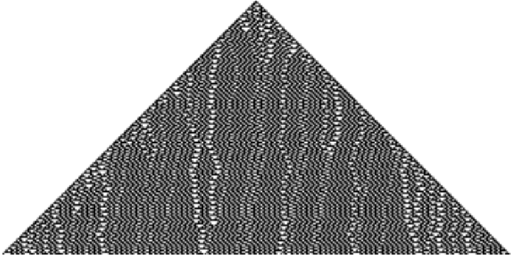
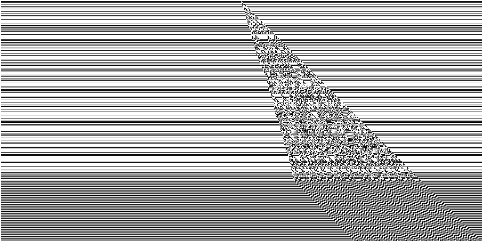
Rules with an odd rule number have the property that black lines across the whole CA can appear whenever that rule is applied. Therefore, if at least one of the rules we combine has an odd rule number, it has an effect if the background cells are counted or not and if the width of the CA is even or odd. Depending on the case the behaviour of the system can be completely different:
As an example we look at the system rule 11 (class 2) and rule 28 (class 2). The result of the first case begins like a class 3 system but ends with class 2 behaviour.
For example, the system whose applied rule depends on whether the number of black cells is even or odd would behave differently, when odd rule numbers are involved. More precisely, there are three cases to distinguish:
1) the system is infinite and/or only the cells of the foreground are counted.
2) the system is finite and has an even width, all cells are counted.
3) the system is finite and has an odd width, all cells are counted.
Rules with an odd rule number have the property that black lines across the whole CA can appear whenever that rule is applied. Therefore, if at least one of the rules we combine has an odd rule number, it has an effect if the background cells are counted or not and if the width of the CA is even or odd. Depending on the case the behaviour of the system can be completely different:
As an example we look at the system rule 11 (class 2) and rule 28 (class 2). The result of the first case begins like a class 3 system but ends with class 2 behaviour.
One can easily see, that these systems are completely different:
in case 1, the system becomes periodic after 558 steps, the evaluation of cases 2 and 3 remains chaotic for a much longer evaluation (it is not known, if they ever become periodic). Note also the obviously different behavior at the left hand side in cases 2 and 3.
in case 1, the system becomes periodic after 558 steps, the evaluation of cases 2 and 3 remains chaotic for a much longer evaluation (it is not known, if they ever become periodic). Note also the obviously different behavior at the left hand side in cases 2 and 3.
Needless to say that differences will also occur (for the same reasons), when the rule depends on the fraction of black cells. But in this case, there are not only three cases but infinitely many - and it occurs for every pair of rule numbers. But this cannot be discussed in detail here.
Effects of Changing a Single Bit in the Initial Condition
Effects of Changing a Single Bit in the Initial Condition
Due to immediate change of the applied rule the change of a single bit in the initial condition will change the global behavior. In opposite to elementary CA, where a changed bit has only local effect which propagate more or less (depending on the rule), there is a huge effect on the whole automaton, if the involved rules are not too simple.
Here are some examples of different behaviour and complexity:
rule 11 and rule 28:
random initial condition:
same random initial condition, one bit changed:
Image difference of the first two images:
The same for rule combination 110-124
Simple Mirrored Rules Yield Complex Behaviour
Simple Mirrored Rules Yield Complex Behaviour
We consider a special group of rules, those where one rule of the CA is exactly the “mirrored” rule of the second one. One could suspect that the CA generated this way behave only very regularly because they basically use “only themselves” and nothing new is generated. However, a systematic search of the 128 (ignoring symmetry) possible combinations shows very interesting examples such as the following:
rule 9 (class 2) and rule 65 (class 2), result: (class 2)
rule 61 (class 2) and rule 103 (class 2), result: (class 4 or class 3, difficult to determine)
rule 62 (class 2) and rule 118 (class 2), result: (class 4 or class 2, difficult to determine)
rule 30 (class 3) and rule 86 (class 3): result: (class 3)
rule 110 (class 4) and rule 124 (class 4): result: (class 3)
The following code can be used to perform the search for mirrored rules.
Conclusion
Conclusion
We have observed some very interesting properties of globally controlled CA which usual CA do not share, for example the strong dependence on the parity of rules and automaton width. These imply that the additional structure which we added through combining the rules based on some criterion strongly improves the system's sensitivity to initial conditions and of course the variety of possible systems, however only when the rule decision parameters of the GCCA are in a certain range (outside that range, the statistical values stabilize as above).
Especially interesting is the observation that this effect exists even if the systems of which a GCCA is composed are not very sensitive to initial conditions, meaning that the way in which we combined the rules yields emergent behaviour regarding the sensitivity of CA to initial conditions. Also, we have found examples of class 2 which, when combined, give class 3 or 4 CA and also examples where GCCA composed of class 4 automata show class 3 behaviour.
Especially interesting is the observation that this effect exists even if the systems of which a GCCA is composed are not very sensitive to initial conditions, meaning that the way in which we combined the rules yields emergent behaviour regarding the sensitivity of CA to initial conditions. Also, we have found examples of class 2 which, when combined, give class 3 or 4 CA and also examples where GCCA composed of class 4 automata show class 3 behaviour.
Keywords
Keywords
◼
Cellular Automaton
◼
Global Control
◼
A New Kind of Science
Acknowledgment
Acknowledgment
I want to thank Stephen Wolfram for let me work on this very interesting project whose original idea is based on a discussion between Stephen Wolfram and Paul Davies in 2003 (see the first reference for more details). I also want to thank my mentor Marco Thiel for many helpful discussions. Furthermore, I want to thank Jesse Friedman, Silvia Hao, Carlos Muñoz, Daniel Sanchez, Nikolay Murzin and Samuele Mongodi for help on my project related chat questions. Finally, I want to thank Yorick Zeschke for his really important help at the last day before project submission.
References
References
◼
Stephen Wolfram (2002), A new kind of science, Wolfram Media