ABSTRACT (original article): Two novel frameworks for handling mathematical and physical problems are introduced. The first, the emerging Jordan form, generalizes the concept of the Jordan canonical form, a well-established tool of linear algebra. The second, dual Jordan quantum physics, generalizes the framework of quantum physics to one in which the hermiticity postulate is considerably relaxed. These frameworks are then used to resolve some long-outstanding problems in theoretical physics, coming from critical statistical models and conformal field theory. I describe these problems and the difficulties involved in finding satisfactory solutions, then show how the concepts of emerging Jordan forms and dual Jordan quantum physics are naturally suited to overcoming these difficulties. Although their applications in this work are limited in scope to rather specific problems, the frameworks themselves are completely general, and I describe ways in which they may be used in other areas of mathematics and physics. Several appendices close the work, which include improvements to a widely used computational algorithm and corrections to some published data. CITATION (original article): Lawrence Liu, Emerging Jordan forms, with applications to critical statistical models and conformal field theory, arXiv:2403.09881. https://doi.org/10.48550/arXiv.2403.09881
Background
Background
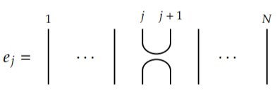
In terms of generators and relations, various algebras to which the name “Temperley--Lieb” (TL) is associated begin with generators subject to relations
{}
e
j
2
e
j
e
j
(
1
)e
j
e
j+1
e
j
e
j
(
2
)e
j
e
k
e
k
e
j
j-k>1
(
3
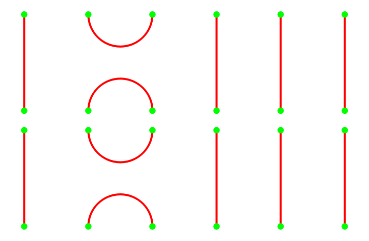
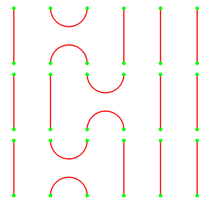
)where the indices take integer values from to , with a fixed integer, is a scalar, and each pair of values for and defines a different algebra. These relations are typically illustrated using diagrams for the generators. To represent generator , on two horizontal rows of points each, connect the neighboring pairs at and , and vertically match all other pairs:(* N -> L *)When two generators are multiplied, the corresponding diagram is obtained following certain rules: stack the diagrams from top to bottom (corresponding to left to right multiplication) and eliminate internal sites, replace closed loops with a numerical factor , and straighten out the curves that connect vertically. In any diagram of the algebra, the lines that connect from top to bottom (rather than between two sites in the same horizontal row) are called through-lines, and the sites to which they are connected are called free. The identity element consists of a diagram with all vertical pairs of sites connected by straight through-lines. It can be shown formally that this algebra of diagrams is isomorphic to the abstract Temperley--Lieb algebra defined by generators and relations (Ridout and Saint-Aubin, 2014). A basis for this algebra is the set of all isotopically distinct diagrams---pairings of two rows of points each without crossings---that can be obtained by repeated multiplication of the generators.The following diagrams for represent the first two relations. The first represents , and when the closed loop in the middle is replaced by , one obtains . The second is , and by “pulling the slack” out of string 4, one recovers . Finally, it is clear that when the pairings in the generators are more than one site away, the multiplication commutes.
1
L-1
L
m
L
m
e
j
L
j
j+1
m
L
L
L=6
e
2
e
2
m
m
e
2
e
2
e
3
e
2
e
2
In[]:=
GraphicsColumn[{Graphics[{Thick,Red,Circle[{3/2,0},1/2,{-π,0}],Circle[{3/2,-3/2},1/2,{0,π}],Line[{{0,0},{0,-3/2}}],Line[{{3,0},{3,-3/2}}],Line[{{4,0},{4,-3/2}}],Line[{{5,0},{5,-3/2}}],Green,Disk[Table[{i,0},{i,0,5}],0.05],Disk[Table[{i,-3/2},{i,0,5}],0.05]}],Graphics[{Thick,Red,Circle[{3/2,0},1/2,{-π,0}],Circle[{3/2,-3/2},1/2,{0,π}],Line[{{0,0},{0,-3/2}}],Line[{{3,0},{3,-3/2}}],Line[{{4,0},{4,-3/2}}],Line[{{5,0},{5,-3/2}}],Green,Disk[Table[{i,0},{i,0,5}],0.05],Disk[Table[{i,-3/2},{i,0,5}],0.05]}]},Spacings->0]
Out[]=
In[]:=
GraphicsColumn[{Graphics[{Thick,Red,Circle[{3/2,0},1/2,{-π,0}],Circle[{3/2,-3/2},1/2,{0,π}],Line[{{0,0},{0,-3/2}}],Line[{{3,0},{3,-3/2}}],Line[{{4,0},{4,-3/2}}],Line[{{5,0},{5,-3/2}}],Green,Disk[Table[{i,0},{i,0,5}],0.05],Disk[Table[{i,-3/2},{i,0,5}],0.05]}],Graphics[{Thick,Red,Circle[{5/2,0},1/2,{-π,0}],Circle[{5/2,-3/2},1/2,{0,π}],Line[{{1,0},{1,-3/2}}],Line[{{4,0},{4,-3/2}}],Line[{{5,0},{5,-3/2}}],Line[{{0,0},{0,-3/2}}],Green,Disk[Table[{i,0},{i,0,5}],0.05],Disk[Table[{i,-3/2},{i,0,5}],0.05]}],Graphics[{Thick,Red,Circle[{3/2,0},1/2,{-π,0}],Circle[{3/2,-3/2},1/2,{0,π}],Line[{{0,0},{0,-3/2}}],Line[{{3,0},{3,-3/2}}],Line[{{4,0},{4,-3/2}}],Line[{{5,0},{5,-3/2}}],Green,Disk[Table[{i,0},{i,0,5}],0.05],Disk[Table[{i,-3/2},{i,0,5}],0.05]}]},Spacings->0]
Out[]=
A simple generalization is to adjoin a generator and site , and to identify site with site , thereby obtaining a periodic Temperley--Lieb algebra. The sites in the top and bottom rows can be thought of as being placed on the inner and outer boundaries of an annulus, evenly spaced, and multiplication consists of nesting two annuli after rescaling one so that its inner boundary matches the outer boundary of the other. In both cases the accessible diagrams consist of planar pairings of points using curves that do not intersect. As before, the curves that join points on the inner boundary to points on the outer boundary of the annulus are called through-lines. We may also depict the multiplication more conveniently using rectangles whose left and right boundaries are identified.
For the periodic case, it is possible for noncontractible closed curves to form that circle the annulus (this requires to be even). These will be given the same weight as contractible loops, although one may consider giving contractible and noncontractible loops different weights---with interesting consequences. Hereafter, we consider only the periodic case in which is even.
e
L
L+1
L+1
1
L
For the periodic case, it is possible for noncontractible closed curves to form that circle the annulus (this requires
L
m
L
Loop representation
Loop representation
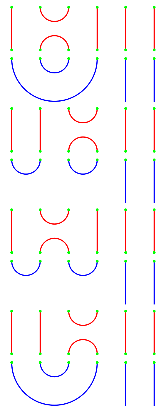
The most natural representations of the TL and periodic TL algebras are given in terms of “link states,” which can be thought of as the basis diagrams cut in half across the through-lines. They consist of single rows of points, some of which are paired below the row, and others with a string attached at one end, such that paths do not cross. The free strings must not be enclosed by pairs, and they are also called through-lines; two examples of link states for follow.
L
L=6
In[]:=
Graphics[{Thick,Blue,Circle[{3/2,0},1/2,{-π,0}],Circle[{3/2,0},3/2,{-π,0}],Line[{{4,0},{4,-3/2}}],Line[{{5,0},{5,-3/2}}],Green,Disk[Table[{i,0},{i,0,5}],0.05]}]Graphics[{Thick,Blue,Circle[{1/2,0},1/2,{-π,0}],Circle[{5/2,0},1/2,{-π,0}],Line[{{4,0},{4,-3/2}}],Line[{{5,0},{5,-3/2}}],Green,Disk[Table[{i,0},{i,0,5}],0.05]}]
Out[]=
Out[]=
Calling the top diagram and the bottom , we see that a=ma, b=mb, b=a, and a=b (in all cases, one pulls the slack out of the strings to get just the pairings). Therefore, we see that in the basis of link states, the diagrams of the TL algebra can be represented by matrices.
a
b
e
2
e
3
e
2
e
3
In[]:=
GraphicsColumn[{Graphics[{Thick,Red,Circle[{3/2,0},1/2,{-π,0}],Circle[{3/2,-3/2},1/2,{0,π}],Line[{{0,0},{0,-3/2}}],Line[{{3,0},{3,-3/2}}],Line[{{4,0},{4,-3/2}}],Line[{{5,0},{5,-3/2}}],Green,Disk[Table[{i,0},{i,0,5}],0.05],Disk[Table[{i,-3/2},{i,0,5}],0.05]}],Graphics[{Thick,Blue,Circle[{3/2,0},1/2,{-π,0}],Circle[{3/2,0},3/2,{-π,0}],Line[{{4,0},{4,-3/2}}],Line[{{5,0},{5,-3/2}}],Green,Disk[Table[{i,0},{i,0,5}],0.05]}],Graphics[{Thick,Red,Circle[{5/2,0},1/2,{-π,0}],Circle[{5/2,-3/2},1/2,{0,π}],Line[{{1,0},{1,-3/2}}],Line[{{4,0},{4,-3/2}}],Line[{{5,0},{5,-3/2}}],Line[{{0,0},{0,-3/2}}],Green,Disk[Table[{i,0},{i,0,5}],0.05],Disk[Table[{i,-3/2},{i,0,5}],0.05]}],Graphics[{Thick,Blue,Circle[{1/2,0},1/2,{-π,0}],Circle[{5/2,0},1/2,{-π,0}],Line[{{4,0},{4,-3/2}}],Line[{{5,0},{5,-3/2}}],Green,Disk[Table[{i,0},{i,0,5}],0.05]}],Graphics[{Thick,Red,Circle[{3/2,0},1/2,{-π,0}],Circle[{3/2,-3/2},1/2,{0,π}],Line[{{0,0},{0,-3/2}}],Line[{{3,0},{3,-3/2}}],Line[{{4,0},{4,-3/2}}],Line[{{5,0},{5,-3/2}}],Green,Disk[Table[{i,0},{i,0,5}],0.05],Disk[Table[{i,-3/2},{i,0,5}],0.05]}],Graphics[{Thick,Blue,Circle[{1/2,0},1/2,{-π,0}],Circle[{5/2,0},1/2,{-π,0}],Line[{{4,0},{4,-3/2}}],Line[{{5,0},{5,-3/2}}],Green,Disk[Table[{i,0},{i,0,5}],0.05]}],Graphics[{Thick,Red,Circle[{5/2,0},1/2,{-π,0}],Circle[{5/2,-3/2},1/2,{0,π}],Line[{{1,0},{1,-3/2}}],Line[{{4,0},{4,-3/2}}],Line[{{5,0},{5,-3/2}}],Line[{{0,0},{0,-3/2}}],Green,Disk[Table[{i,0},{i,0,5}],0.05],Disk[Table[{i,-3/2},{i,0,5}],0.05]}],Graphics[{Thick,Blue,Circle[{3/2,0},1/2,{-π,0}],Circle[{3/2,0},3/2,{-π,0}],Line[{{4,0},{4,-3/2}}],Line[{{5,0},{5,-3/2}}],Green,Disk[Table[{i,0},{i,0,5}],0.05]}]},Spacings->0]
Out[]=
Because the number of link states grows exponentially with the number of sites, we will use different numerical representations of the link states in Mathematica for different computational purposes, in order to increase efficiency and the number of sites we can handle.
We can convert from the binary notation to the pairing notation as follows. Index the sites by their position, and iteratively remove 1-0 pairs that represent pairings; whatever remains when only 1s are left are through-lines. As an illustrative example on 8 sites:
One then identifies a state with its image under this map. In algebraic terms, one takes a quotient by an equivalence relation whose equivalence classes are the preimages of the planar diagrams under this mapping. In Mathematica, this mapping is accomplished most simply by sorting the pairs in ascending order (the function takes as an argument a base-10 numeric representation of a link state and returns the same):
loopDim is the number of basis states, and pos gives the ordinal position of a state within the basis.
The relations between the link state representations and their properties discussed so far are summarized in the following diagram. Blue arrows indicate conversions between representations, while red arrows indicate computed properties.
“num” refers to the numeric representation and “inv” the inverse. We may now check relations (1)--(3):
In the periodic TL algebra, the following relations are obeyed by the (abstract) generators:
Supersymmetric representation
Supersymmetric representation
Check that this is indeed a subspace:
With an eye on what follows, the basis is stored as a positively-indexed version and a negatively-indexed version, with a corresponding sign for the basis element. For instance, if pos[m] gives n then pos[-m] gives -n.
We see that shifting some basis vectors results in the negative of another.
Conformal Field Theory
Conformal Field Theory
The supersymmetric Hamiltonian contains the eigenvalues of the loop Hamiltonian, with additional multiplicities and values. They are due to the fact that the Hilbert space of the supersymmetric spin chain contains multiple copies of the loop representation modules and generating functions, as well as additional modules not mentioned here.
CITE THIS NOTEBOOK
CITE THIS NOTEBOOK
Emerging Jordan forms, with applications to critical statistical models and conformal field theory
by Lawrence Liu
Wolfram Community, STAFF PICKS, July 2, 2024
https://community.wolfram.com/groups/-/m/t/3203445
by Lawrence Liu
Wolfram Community, STAFF PICKS, July 2, 2024
https://community.wolfram.com/groups/-/m/t/3203445