ABSTRACT (original article): Integrals to calculate generalised magnetic coordinates from an input magnetic flux function asymptotically close to the separatrix are presented, and implemented in the GPEC/DCON code suite. These integrals allow characterisation of the magnetic equilibrium of a diverted tokamak, in magnetic coordinates, arbitrarily close to the last closed flux surface, avoiding the numerical issues associated with calculating diverging field-line integrals near a magnetic x-point. These methods may assist ongoing efforts to develop robust asymptotic equilibrium behaviour for spectral 3D MHD codes at the separatrix. CITATION (original article): S Benjamin et al 2025, Computation of generalised magnetic coordinates asymptotically close to the separatrix, Plasma Phys. Control. Fusion 67 065019. https://doi.org/10.1088/1361-6587/add9ca
Introduction
Introduction
In this paper, a number of analytic and numerical calculations were conducted to investigate how we can more efficiently describe the mathematical structure of magnetic X-points during tokamak stability calculations. The Mathematica scripts used in that study have been collated here into a single document, intended to be used as a supplement to the full article; throughout the document, any named equations and figures refer to those in the article.
Defining local coordinates
Defining local coordinates
In this section we compute a transformed coordinate frame following Sec. 3.2 of the article.
As per Eqs. 13 & 14:
As per Eqs. 13 & 14:
In[]:=
xtest[Rloc_,Zloc_,ϑ_]:=Cos[ϑ]*Rloc+Sin[ϑ]*Zlocytest[Rloc_,Zloc_,ϑ_]:=-Sin[ϑ]*Rloc+Cos[ϑ]*Zloc
Using this to express , in terms of x, y:
R
local
Z
local
In[]:=
FullSimplify[Solve[xt==xtest[Rloc,Zloc,ϑ]&&yt==ytest[Rloc,Zloc,ϑ],{Rloc,Zloc}]]
Out[]=
{{RlocxtCos[ϑ]-ytSin[ϑ],ZlocytCos[ϑ]+xtSin[ϑ]}}
Defining , coordinates using the above result:
R
local
Z
local
In[]:=
R=Rx+Rlocal;Rlocal=x*Cos[ϑ]-y*Sin[ϑ];Zlocal=y*Cos[ϑ]+x*Sin[ϑ];
Printing in terms of x, y, ϑ, and major radius of X-point (). This will come in handy later...
R
local
R
X
In[]:=
R
Out[]=
Rx+xCos[ϑ]-ySin[ϑ]
We now define x, y local coordinates in terms of local polar coordinate system ν, ρ (Eq. 31):
In[]:=
x[r_,θ_]:=r*Cos[θ]y[r_,θ_]:=r*Sin[θ]
We define coordinate χ (see Fig. 6) in terms of Cartesian x, y:
In[]:=
χcart[x_,y_,γ_]:=-Cos[γ]*x+Sin[γ]*y
We calculate the ∇χ direction, in terms of Cartesian x, y:
In[]:=
Nablaχcart[x_,y_,γ_]:={D[χcart[x1,y1,γ],x1],D[χcart[x1,y1,γ],y1]}/.{x1->x,y1->y};Nablaxcart={1,0};Nablaχcart[0,0,γ]
Out[]=
{-Cos[γ],Sin[γ]}
We also must calculate the ∇x direction:
In[]:=
Nablaxcart={1,0};
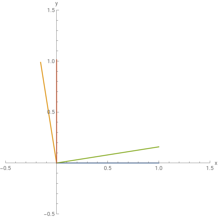
We can now illustrate our new coordinate vectors such as ∇χ on the x-y axes, (assuming we have solved for the angle between separatrix legs γ0):
γ0=.45*Pi;ListLinePlot{{{0,0},Nablaxcart},{{0,0},Nablaχcart[0,0,γ0]},{{0,0},{1,Cot[γ0]}},{{0,0},{0,Csc[γ0]}}},
Out[]=


Visualising the lowest order Taylor expansion of ψ
Visualising the lowest order Taylor expansion of ψ
In this section we visualise the ψ function near the magnetic X-point, and confirm some aspects of the Taylor-expansion description of ψ that are relevant to Eq. 15, and appendix section A.3.
We start by choosing a set of inputs that define the x-point, such as the angle γ (see Fig. 6) and lowest order coefficient c11 (Eq. 15).
In[]:=
Ψsep=0;γ0=.45*Pi;c110=-1;
Now, we write out the lowest order expansion of ψ = (Eq. 15):
ψ
11
In[]:=
ψ11[x_,χ_,c11_]:=Ψsep+c11*x*χψ11γ[x_,y_,γ_,c11_]:=ψ11[x,χcart[x,y,γ],c11]
By including higher order terms, we can simulate a more general ψ, for comparison’s sake:
In[]:=
ψ[x_,χ_,c11_]:=Ψsep+c11*x*χ+0.233*x^2*χ-3*x*χ^3ψγ[x_,y_,γ_,c11_]:=ψ[x,χcart[x,y,γ],c11]
We calculate the ∇ψ direction:
In[]:=
Nablaψcart[x_,y_,γ_,c11_]:=(D[ψ[x1,χ1,c11],x1]*Nablaxcart+D[ψ[x1,χ1,c11],χ1]*Nablaχcart[x,y,γ])/.{x1->x,χ1->χcart[x,y,γ]};
We calculate (∇ψ · ∇ρ)/(|∇ψ||∇ρ|) - the normalised radial projection of ∇ψ:
In[]:=
NablaψdotρNORM[x_,y_,γ_,c11_]:=Dot[Nablaψcart[x,y,γ,c11],{x,y}]/(Norm[Nablaψcart[x,y,γ,c11]]*Norm[{x,y}])
We allow the use of polar input coordinates for plotting:
In[]:=
NablaψdotρNORMPOLAR[r_,θ_,γ_,c11_]:=NablaψdotρNORM[x[r,θ],y[r,θ],γ,c11]NablaψdotρNORMν[r_,ν_,γ_,c11_]:=NablaψdotρNORMPOLAR[r,-ν+Pi/2,γ,c11]
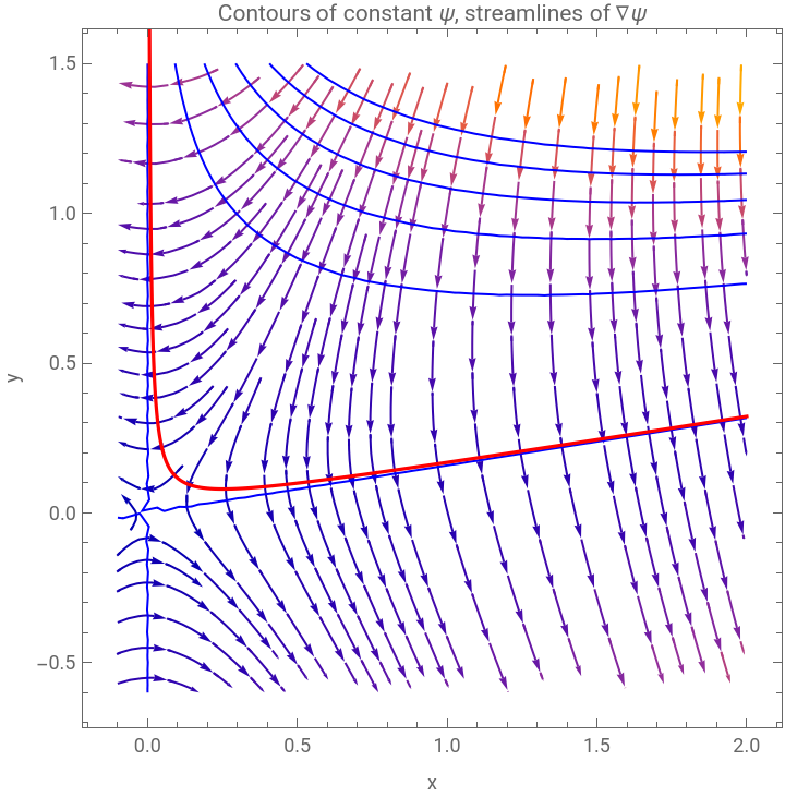
In the following plot, we show the behaviour of ∇ψ in the vicinity of the X-point.
ShowStreamPlot[Nablaψcart[x,y,γ0,c110],{x,-0.1,2},{y,-0.6,1.5}],ContourPlotψγ[x,y,γ0,c110],{x,-0.1,2},{y,-0.6,1.5},,ParametricPlotx,+x*Cot[γ0],{x,0.00000001,2},,FrameLabel->{"x","y"},PlotLabel->"Contours of constant ψ, streamlines of ∇ψ"
0.01
x
Out[]=
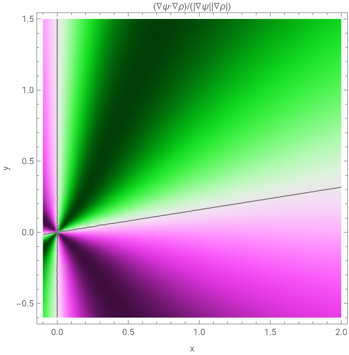
Now we plot (∇ψ · ∇ρ)/(|∇ψ||∇ρ|) in the vicinity of the X-point.
DensityPlotNablaψdotρNORM[x,y,γ0,c110],{x,-0.1,2},{y,-0.6,1.5},
Out[]=
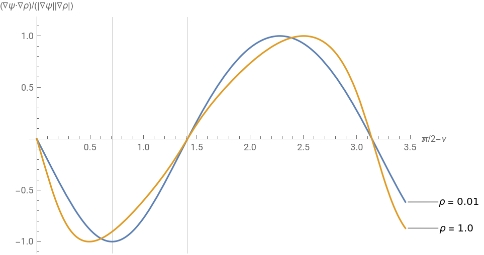
In the following plot, we compute (∇ψ · ∇ρ)/(|∇ψ||∇ρ|) over an arc in ν, at some large radius (ρ2 = 1) versus a smaller radius (ρ1 = 0.01). ψ’s behaviour approaches that of at small radius; we see that ∇ψ is entirely pointing in the ∇ρ direction (such that (∇ψ · ∇ρ)/(|∇ψ||∇ρ|)=1, ∇ψ · ∇ν = 0) at ν ≈ /2. For , (∇ψ · ∇ρ)/(|∇ψ||∇ρ|) = -1 at exactly ν = /2.
ψ
11
γ
ψ
11
γ
Plot{NablaψdotρNORMν[0.01,ν,γ0,c110],NablaψdotρNORMν[1,ν,γ0,c110]},{ν,0,1.1Pi},Print["Vertical lines represent γ0/2, γ0."]
Out[]=
Solving for field line trajectories
Solving for field line trajectories
We can calculate the relationship y(x) by setting dy/dx = vy/vx, then integrating with respect to x:
Since the red line (Eq. 17) and the dotted line (level-set of ψ) match, we are satisfied.
Deriving equation 18
Deriving equation 18
We can use Mathematica to help us simplify this expression as follows:
After re-arranging the log, the above gives us Eq. 19, the solution given in the article.
and in the general case:
Only the former two cases were presented in the article.
We calculate the normalised difference between the Mathematica values and those from the GPEC/DCON integration scripts, as distance from the separatrix is varied:
For detailed scans of the convergence of these integrals, please see the full article here https://doi.org/10.1088/1361-6587/add9ca.
CITE THIS NOTEBOOK
CITE THIS NOTEBOOK
Computation of generalised magnetic coordinates asymptotically close to the separatrix
by Stuart Benjamin
Wolfram Community, STAFF PICKS, February 11, 2026
https://community.wolfram.com/groups/-/m/t/3638679
by Stuart Benjamin
Wolfram Community, STAFF PICKS, February 11, 2026
https://community.wolfram.com/groups/-/m/t/3638679