This notebook builds a stage-wise (tanks-in-series) equilibrium model of a chromatography column and uses it both to generate synthetic data and to recover the model's parameters from that data.
The column is discretized into 50 well-mixed equilibrium stages. For two solutes A and B, each governed by its own linear equilibrium constant (KA, KB), a system of first-order ODEs describing stage-to-stage concentration transfer is assembled and solved with NDSolve for a rectangular pulse injection at the column inlet. The resulting exit-concentration profile from the final stage is sampled over time and corrupted with uniform random noise to produce a synthetic "noisy chromatogram", mimicking real detector data.
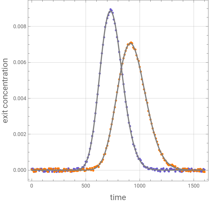
The noisy data is then fed into NonlinearModelFit (using the interior-point method, with bounds around the true KA/KB values) to re-estimate the equilibrium constants from the simulated measurements, and the fitted model is compared against the noisy data and the noise-free simulation to check how well the original parameters are recovered.
Equilibrium constants
In[]:=
KA=0.9;KB=1.3;
Total volume
In[]:=
V
tot
50 well-mixed stirred tanks or 50 perfect equilibrium stages
In[]:=
NS=50;
Stage volume
In[]:=
V
stage
V
tot
Volumetric flow rate
In[]:=
L=0.4;
Void fraction
In[]:=
ϵ=0.4;
Column diameter
In[]:=
Dc=4;
Column length
In[]:=
Lbed=25;
Governing equations
In[]:=
eq[i_]:=D[[t],{t,1}]L([t]-[t])ϵ+(1-ϵ)KA;eq2[i_]:=D[[t],{t,1}]L([t]-[t])ϵ+(1-ϵ)KB;eqn=Table[eq[i],{i,1,50}];
CA
i
CA
i-1
CA
i
V
stage
V
stage
CB
i
CB
i-1
CB
i
V
stage
V
stage
In[]:=
initialCond=Table[[0]0,{i,1,50}];sys=Flatten[Join[eqn,initialCond]];Unknown=Table[,{i,1,50}];eqn2=Table[eq2[i],{i,1,50}];initialCond2=Table[[0]0,{i,1,50}];sys2=Flatten[Join[eqn2,initialCond2]];Unkn2=Table[,{i,1,50}];
CA
i
CA
i
CB
i
CB
i
Rectangular pulse injection at the column inlet
In[]:=
CA
0
CA
init
CA
init
CB
0
CB
init
CB
init
In[]:=
sol1=NDSolve[sys,Unknown,{t,0,5000}];sol2=NDSolve[sys2,Unkn2,{t,0,3000}];
Generate synthetic noisy chromatogram using exit concentrations of species A and B
In[]:=
datareal1=Table[{i,First[Evaluate[[t]]/.sol1/.t->i]+0.0001RandomReal[{-1,1}]},{i,0,1600,10}];
CA
50
In[]:=
datareal2=Table[{i,First[Evaluate[[t]]/.sol2/.t->i]+0.0001RandomReal[{-1,1}]},{i,0,1600,10}];
CB
50
p1=ListPlot{datareal1,datareal2},
Out[]=
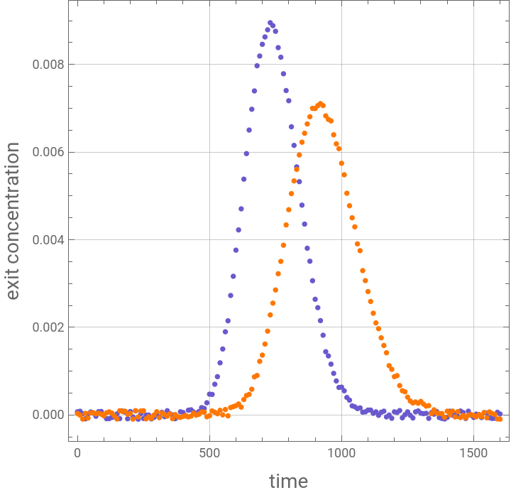


Use the synthetic noisy chromatogram to fetch KA and KB (the equilibrium constants). To do so, we use ParametricNDSolveValue and NonlinearModelFit
In[]:=
Clear[KA,KB]
In[]:=
SYS=Join[sys,sys2];
In[]:=
Length@SYS
Out[]=
200
In[]:=
UNK=Join[Unknown,Unkn2];
In[]:=
Length@UNK
Out[]=
100
In[]:=
pfunall=ParametricNDSolveValue[SYS,UNK,{t,0,2000},{KA,KB}]
Out[]=
ParametricFunction


Defining the model input for NonlinearModelFit command
model[KA_,KB_][i_,t_]:=Through[pfunall[KA,KB][t],List][[i]]/;And@@NumericQ/@{KA,KB,i,t};
In[]:=
datanoisy=Flatten[Join[{Table[{50,datareal1[[i]][[1]],datareal1[[i]][[2]]},{i,41,Length[datareal1]}],Table[{100,datareal2[[i]][[1]],datareal2[[i]][[2]]},{i,41,Length[datareal2]}]}],1];
In[]:=
Length@datanoisy
Out[]=
242
In[]:=
fit=NonlinearModelFit[datanoisy,{model[KA,KB][i,t],1.0>KA>0.8&&1.4>KB>1.2},{KA,KB},{i,t},Method->"InteriorPoint"](*callingtheNonlinearModelFitcommandandgatheringrelevantstatisticaldata*)
Out[]=
FittedModel
In[]:=
nlm=Normal@fit
Out[]=
model[0.979998,1.38][i,t]
In[]:=
Total[fit["FitResiduals"]^2]
Out[]=
7.77464×
-7
10
In[]:=
p3=Plot[{model[0.979998,1.38][50,t],model[0.979998,1.38][100,t]},{t,0,1600},PlotStyle->Gray];
In[]:=
Show[p1,p3]
Out[]=
CITE THIS NOTEBOOK
CITE THIS NOTEBOOK
Recovering equilibrium constants from simulated noisy chromatography data
by Housam Binous
Wolfram Community, STAFF PICKS, August 30, 2026
https://community.wolfram.com/groups/-/m/t/3789514
by Housam Binous
Wolfram Community, STAFF PICKS, August 30, 2026
https://community.wolfram.com/groups/-/m/t/3789514