ABSTRACT (original article): Shaping the animal body plan is a complex process that involves the spatial organization and patterning of the different germ layers. Recent advances in live imaging have started to unravel the cellular choreography underlying this process in mammals, however, the sequence of events transforming an unpatterned cell ensemble into structured territories is largely unknown. Here, using gastruloids –3D aggregates of mouse embryonic stem cells- we study the formation of one of the three germ layers, the endoderm. We show that the endoderm is generated from an epiblast-like homogeneous state by a three-step mechanism: (i) a loss of E-cadherin mediated contacts in parts of the aggregate leading to the appearance of islands of E-cadherin expressing cells surrounded by cells devoid of E-cadherin, (ii) a separation of these two populations with islands of E-cadherin expressing cells flowing toward the aggregate tip, and (iii) their differentiation into an endoderm population. During the flow, the islands of E-cadherin expressing cells are surrounded by cells expressing T-Brachyury, reminiscent of the process occurring at the primitive streak. Consistent with recent in vivo observations, the endoderm formation in the gastruloids does not require an epithelial-to-mesenchymal transition, but rather a maintenance of an epithelial state for a subset of cells coupled with fragmentation of E-cadherin contacts in the vicinity, and a sorting process. Our data emphasize the role of signaling and tissue flows in the establishment of the body plan. CITATION (original article): Ali Hashmi, Sham Tlili, Pierre Perrin, Molly Lowndes, Hanna Peradziryi, Joshua M Brickman, Alfonso Martínez Arias, Pierre-François Lenne (2022) Cell-state transitions and collective cell movement generate an endoderm-like region in gastruloids eLife 11:e59371. DOI: https://doi.org/10.7554/eLife.59371
Gastruloid 1: segmenting gastruloids and quantifying morphology
Gastruloid 3: tracking bulk motion of cells
Gastruloid 1: segmenting gastruloids and quantifying morphology
Gastruloid 3: tracking bulk motion of cells
Functions definitions
Functions definitions
Section 1: neighbourhood analysis of a single gastruloid
Section 1: neighbourhood analysis of a single gastruloid
Rationale: A gastruloid is composed of several hundred cells. For the purpose of my research question it was important to know the various cell types that exist in the gastruloid at different time points. For instance, we can look at the gastruloid at the third day or 72 hours of development; we observe three different cell populations namely titled as ‘EB’, ‘B’ or ‘E’ from now onwards. The populations are titled based on the kind of important proteins/factors that the cell is ‘expressing’ or producing (here the two factors under consideration are E-cadherin and Brachyury).
‘EB’ refers to cell population that expresses both E-cadherin and Brachyury. ‘B’ and ‘E’ populations refer to cells that express Brachyury and E-cadherin respectively, but not both. It is critical to determine how the different cell populations are distributed in space and how homogeneous or fragmented the populations are. This gives an idea of how the different cell types interact with each other over time, and whether they affect one another.
Below we import the cell centroids from a single gastruloid and plot the centroids as spheres in space .
In[]:=
{type,slice,X,Y,V,Cpos,Z,T,Xmic,Ymic,Zmic}=Transpose@Import["C:\\Users\\hashmial\\Downloads\\notebook2\\populationdist.csv","Data"];Counts[Rest@type]
Out[]=
181,231,34,42
In[]:=
{div,ecadbrach,brach,ecad}=Transpose[{Extract[Xmic,#],Extract[Ymic,#],Extract[Zmic,#]}]&/@{Position[type,4],Position[type,1],Position[type,2],Position[type,3]};
colour=Lighter@Blue,,Lighter@Green;Graphics3D[{colour[[1]],Sphere[#,3.5]&/@ecadbrach,colour[[2]],Sphere[#,3.5]&/@brach,colour[[3]],Sphere[#,3.5]&/@ecad},BoxedTrue,ImageSizeMedium,BackgroundNone,Lighting"Neutral"]

Out[]=

The gray coloured cells represent the ‘B’ cell population whereas the blue and green coloured cells represent the ‘EB’ and ‘E’ cell populations respectively. The cell centroid positions have been rescaled to fit a unit-sphere. This can later help us to pool data and perform analysis on multiple such gastruloids (see section 2)
In[]:=
populationCells=ecadbrach~Join~brach~Join~ecad;cent=Mean@populationCells;lmax=Max[Norm[#-cent]&/@populationCells];populationCellsRescale=(#-cent)/lmax&/@populationCells;
In[]:=
iden=Join[ConstantArray["EB",Length@ecadbrach],ConstantArray["B",Length@brach],ConstantArray["E",Length@ecad]];
In[]:=
Graphics3D[{{Opacity[0.1],Gray,Sphere[]},{Opacity[0.7],Ball[#,0.07]&/@populationCellsRescale}},ImageSize->Medium]
Out[]=

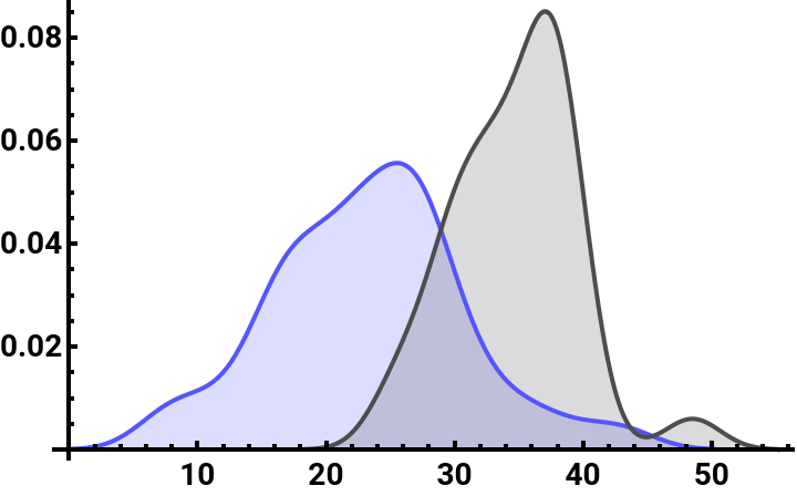
We determine the distance of how the two cell populations are distributed in space about the mean position of the gastruloid. We observe below that the ‘B’ cell population is distributed more on the periphery of the gastruloid while the ‘EB’ cell population is more confined towards the centre.
In[]:=
polarDistcells=With[{cent=Mean@populationCells},{(xcoordTrans[x-cent])/@ecadbrach,(xcoordTrans[x-cent])/@brach}];
In[]:=
SmoothHistogram[polarDistcells[[All,All,1]],Automatic,"PDF",PlotStyle->{Lighter@Blue,colour[[2]]},PlotLegends->{Style["EB",Bold,Black],Style["B",Bold,Black]},Filling->Axis,AxesStyle->{{Black,Thick},{Black,Thick}},TicksStyle->Directive["Label",Bold,14]]
Out[]=


We can analyse the neighbourhood of the different cell populations, for instance, what cell type surrounds a specific cell type and how fragmented the various cell populations are within the gastruloid. We do this by converting the cell centroid distribution to a Delaunay mesh.
In[]:=
(*DelaunayMesh*)assoc=Join[<|Thread[ecadbrach"EB"],Thread[brach"B"],Thread[ecad"E"]|>];pts=Join[ecadbrach,brach,ecad];mesh=DelaunayMesh[pts]
Out[]=

In[]:=
graph=Graph3D[MeshPrimitives[mesh,1]/.Line[{x_,y_}]UndirectedEdge[x,y],VertexStyleJoin[Thread[brachRed],Thread[ecadGreen]]]
Out[]=

colkeys=MapAtN,Thread[brachcolour[[3]]]~Join~Thread[ecadbrachLighter@Blue]~Join~Threadbrach~Join~Thread[ecadGreen],{All,1};
In[]:=
Graph3D[MeshPrimitives[mesh,1]/.Line[{x_,y_}]UndirectedEdge[x,y],VertexStylecolkeys]//Rasterize[#,"Image",ImageResolution512,BackgroundNone]&
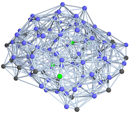
We remove any false edges, where the plausible edges are defined by a threshold that separates two cell centroids from each other. The geometric mesh then is essentially a graph and we can use graph related metrics to define neighbourhoods of cells and furthermore, determine the degree of fragmentation of the three populations
Extract edges less than 12 units
From the results of the adjacency matrix with edge filtering, we see that an ‘EB’ cell type is surrounded by mostly ‘EB’ population whereas a ‘B’ cell type is surrounded by both ‘B’ and ‘EB’ cell population. The third cell type ‘E’ is surrounded by mostly ‘EB’ cell type and by none of its own type.
Below we infer the fragmentation (i.e. size of the connected components) of the three different cell populations
Below we infer the fragmentation (i.e. size of the connected components) of the three different cell populations
Connected components of ‘EB’ population (showing only the EB cell connectivity in space)
Connected components of ‘B’ population (showing only the B cell connectivity in space)
Connected components of ‘E’ population (showing only the E cell connectivity in space)
Section 2: Spatial density map of cell population from pooled gastruloids
Section 2: Spatial density map of cell population from pooled gastruloids
We can pool cell centroids from multiple gastruloids to create a more faithful spatial density map for the distribution of the various cell population.
Spatial distribution of pooled data
Spatial distribution of pooled data
Looking at the projection of the three different cell types (colour-coded) on the x-y-z planes
Creating a statistical data distribution for the various cell types and using it to create a spatial density map of the various cell populations
Computing probability & population fraction
Computing probability & population fraction
We can compute the probability of finding a certain cell type at a given distance from the centre of the gastruloid (assuming cells are distributed in a sphere) using our statistical spatial distribution. We can do it conveniently using the NProbability function with NIntegrate method to find the probability. The probability in finding a specific cell type in a certain radial band (or shell) can then be found by taking differences of probabilities between the extremal points.
Saving results of ‘probball1’ as ‘probball1N’
Probability/Volume multiplied by its weight/population fraction
Saving results of ‘probball2’ as ‘probball2N’
Probability/Volume multiplied by its weight/population fraction
Saving results of ‘probball3’ as ‘probball3N’
Probability/Volume and multiplied by its weight/population fraction
Plotting the population fraction as a function of the radius of the sphere as well as the weighted population distribution. The weight here refers to the (population of a specific cell type/total cell population)
weight*(probability/volume) for the three classes
The ∑ of all the cell population fractions at any given point in space should be 1.
CITE THIS NOTEBOOK
CITE THIS NOTEBOOK
Gastruloid 2: spatial organization of cell population at 72 hours of development
by Ali Hashmi
Wolfram Community, STAFF PICKS, October 11, 2023
https://community.wolfram.com/groups/-/m/t/3032750
by Ali Hashmi
Wolfram Community, STAFF PICKS, October 11, 2023
https://community.wolfram.com/groups/-/m/t/3032750