If we regard interference and entanglement as the most distinctive features of the quantum world, then “which-way” experiments lie at the heart of quantum physics, vividly illustrating the contrast between classical and quantum conceptions of nature. The idea of “which-way” experiments can be traced back to Einstein’s famous proposal of a double-slit experiment with a movable slit at the 1927 Solvay conference, intended to demonstrate an inconsistency in the orthodox (Copenhagen) interpretation of quantum theory. In response, Bohr analyzed this setup within his own interpretation when addressing the Einstein–Podolsky–Rosen (EPR) paradox. Since then, the conceptual and experimental issues surrounding “which-way” experiments have been explored extensively, both theoretically and experimentally, from many different viewpoints.
The central question in “which-way” experiments is: under what conditions does the interference pattern appear or disappear? The presence of an interference pattern is interpreted as evidence of the wave-like nature of quantum systems, while its disappearance is associated with particle-like (corpuscular) behavior. According to Bohr, wave-like and particle-like behaviors are complementary and cannot be observed simultaneously within the same experimental context. Moreover, the storage of path information naturally leads to another central quantum concept: entanglement, which lies at the core of quantum computation. This is one of the reasons why which-way experiments are so interesting, both conceptually and technically.
In this essay, I will review which-way experiments using the formalism and perspective of quantum computation. I will also discuss how quantum erasure can restore interference patterns and briefly examine Bohr’s interpretation of quantum theory, since any attempt to translate the mathematics of quantum theory into words inevitably involves terms and concepts introduced by Bohr. Whether these ideas truly clarify or deepen our understanding of quantum phenomena is, perhaps, a separate question.
What is Copenhagen interpretation?
What is Copenhagen interpretation?
Copenhagen Interpretation of quantum mechanics is a blended heap of different challenging views toward understanding the quantum formalism. Among the famous founders (e.g., Heisenberg, Born, Pauli, Jordan, and others), Bohr was the most influential figure. For this reason—and to clearly distinguish his approach from, for example, the von Neumann influence (i.e., the reduction/collapse of the state function) on what is usually called the Copenhagen interpretation—it is more reasonable to speak simply of Bohr’s Interpretation. However, it is really difficult to talk about a coherent and unique attitude of Bohr toward the foundations of quantum mechanics.
Briefly speaking, Bohr’s interpretation could be described as follows:
Since the phenomena transcend the scope of classical physical explanation, the account of all evidence must be expressed in classical terms. However, it is not possible to use all classical terms in the quantum world in the same way that we use them in classical physics; any given application of classical concepts precludes the simultaneous use of other classical concepts which, in a different connection, are equally necessary for the elucidation of the phenomena. This is what Bohr meant by the Complementarity Principle.
Since the phenomena transcend the scope of classical physical explanation, the account of all evidence must be expressed in classical terms. However, it is not possible to use all classical terms in the quantum world in the same way that we use them in classical physics; any given application of classical concepts precludes the simultaneous use of other classical concepts which, in a different connection, are equally necessary for the elucidation of the phenomena. This is what Bohr meant by the Complementarity Principle.
An adequate tool for a complementary way of description is offered precisely by the quantum-mechanical formalism—which represents a purely symbolic scheme permitting only predictions (along the lines of the correspondence principle) as to results obtainable under conditions specified by means of classical concepts. In Bohr’s view, the quantum formalism is nothing but the mathematical presentation of the Complementarity idea, an idea claimed to be the consistent and rational generalization of classical terms to the quantum realm. The importance of Complementarity in his view is comparable with the position of causality in classical physics, even similar in a philosophical sense.
We should keep in mind that quantum physics just describes phenomena. In the spirit of objective description, the term phenomenon refers only to observations obtained under circumstances whose description includes an account of the whole experimental arrangement. Moreover, we are directly reminded that every atomic phenomenon is “closed” in the sense that its observation is based on registrations obtained by means of suitable amplification devices with irreversible functioning—such as permanent marks on a photographic plate caused by the penetration of electrons into the emulsion. In this connection, it is important to realize that the quantum-mechanical formalism permits well-defined applications referring only to such closed phenomena.
Although Bohr explicitly explained what he meant by phenomenon, there is no consensus on the exact meaning of the Complementarity Principle. This ambiguity is directly related to vagueness in Bohr’s view about the position of classical physics in the quantum realm. We should carefully keep in mind that, in Bohr’s view, an unambiguous, objective, and communicable description of quantum phenomena is only possible with the aid of classical explanations. It could thus be said that Bohr’s view of the quantum domain was a continual traditional view with deep roots in classical physics—in contrast to beliefs in a revolutionary shift.
Let alone the dogmatic aspects of Bohr’s stance in some respects, his interpretation provides a suitable and neat language for communicating the mathematical formalism of quantum mechanics. In other words, it offers a terminology that helps us correctly describe the formalism in words and prevents certain misconceptions. For example, while the Complementarity Principle states that there is a preclusion in the simultaneous possibility of obtaining exact information about complementary properties of a physical system, it does not provide a reason for such a situation, in short, instead of explaining the weirdness of quantum theory, Bohr maintained that it is impossible to do so.
Interference experiment
Interference experiment
Consider a quantum system prepared in a superposition (i.e., linear combination) of two distinguishable states as follows:. The states and can represent, for example, the spin of a spin-1/2 system such as silver atoms, the path of photons in a Mach–Zehnder interferometer, or the wave functions associated with the two paths (slits) in a double-slit Young experiment. In the double-slit case, the corresponding spatial wave functions are (x)=〈x|j〉 with .
|ψ〉=(|0〉+|1〉)
1
2
|0〉
|1〉
ψ
j
j=0,1
For simplicity, we assume that the two states are orthogonal, meaning that their inner product vanishes: . In the spatial representation, this orthogonality condition can be written as where * denotes complex conjugation (for example =Sin[x]-Cos[x]). Since the description in a discrete two-dimensional vector space is simpler, we restrict our discussion to that case. In this representation, the state is given by the unit vector and likewise . It is easy to verify the orthogonality: . The states and are usually called the computational basis; “basis” because they serve as the fundamental vectors spanning the two-dimensional complex vector space (also called the Hilbert space) relevant to the problem we are studying.
〈0|1〉=0
∫x(x)(x)=0
ψ
1
*
ψ
2
*
(Sin[x]+Cos[x])
|0〉
{1,0}
|1〉={0,1}
{0,1}.=0
*
{1,0}
|0〉
|1〉
Let’s revisit what is happening in a simple interference experiment. An individual quantum system is first prepared in the state . We then apply an operator to it (for example, by sending photons through a beam splitter, or particles through a double slit in a Young-type experiment), and the state is transformed into the superposition (|0〉+|1〉). Next, we apply another operation that introduces a phase factor only on the component of the state. This phase shift can be implemented in different physical ways; for instance, for photons by making one arm of a Mach–Zehnder interferometer longer than the other, or by applying an external field only along the path corresponding to in the case of spin-1/2 systems or in a double-slit experiment. Overall, after the phase shifter, the quantum state is transformed into 0+1 with denoting the phase shift. The last operation before the measurement is repeating the same step that prepare the superposition, for example a second beam-splitter in a Mach–Zehnder interferometer. Therefore, the quantum state is transformed into (1+)0+(1-)1.
|0〉
1
2
|1〉
|1〉
1
2
θ
θ
1
2
θ
θ
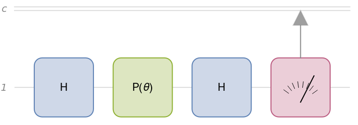
Let’s mimic these steps in a quantum circuit; in other words, the formulation of Mach–Zehnder interferometer in the language of quantum computation. We start by preparing a qubit in a register state. The first Hadamard gate (denoted by H in the circuit diagram) represents the first beam splitter. The phase-shift gate (denoted by P in the circuit diagram) introduces a relative phase, the second Hadamard gate represents the second beam splitter, and finally we perform a measurement. Let’s define the circuit in the Wolfram quantum framework:
In[]:=
ClearAll[θ]$Assumptions=θ∈Reals;qc1=QuantumCircuitOperator[{"H","P"[θ],"H",{1}}];qc1["Diagram"]
Out[]=
Calculate the system evolution through each step:
In[]:=
steps1=ComposeList[Most@qc1["Operators"],QuantumState[]];
In above code, we dropped the measurement (the last step). We shall discuss it very soon.
Show state evolution step by step:
In[]:=
Grid[Prepend[Transpose[{Style[#,Bold]&/@{"Initial state","After 1st Hadamard","After phase shift","After 2nd Hadamard"},TraditionalForm/@steps1,MatrixForm[FullSimplify@Normal@#["StateVector"]]&/@steps1}],Style[#,Bold]&/@{"Step","State in Dirac notation","State vector"}],Frame->All,AlignmentLeft]
Out[]=
Step | State in Dirac notation | State vector | ||
Initial state | |0〉 |
| ||
After 1st Hadamard | 1 2 1 2 |
| ||
After phase shift | 1 2 θ 2 |
| ||
After 2nd Hadamard | 1 2 θ 2 1 2 θ 2 |
|
Now let’s focus on the last step. The measurement step is the most subtle and conceptually challenging part of quantum theory. The evolution (i.e., the transformation of the quantum state) in this step is different from that in all the previous steps. More precisely, all earlier steps follow the Schrödinger equation and are deterministic and unitary, whereas measurement involves a fundamentally random evolution.
If we run the experiment on individual systems (for example, sending atoms or photons one by one through the device) and measure in the computational basis, we will observe either 0 or 1 at random. Quantum theory does not explain how a specific individual outcome is selected in each run, nor why the process is random, but it does fully describe the statistics of the outcomes. In other words, the probabilities of different measurement results are completely determined by quantum theory.
If we run the experiment on individual systems (for example, sending atoms or photons one by one through the device) and measure in the computational basis, we will observe either 0 or 1 at random. Quantum theory does not explain how a specific individual outcome is selected in each run, nor why the process is random, but it does fully describe the statistics of the outcomes. In other words, the probabilities of different measurement results are completely determined by quantum theory.
To calculate the measurement probabilities, we first determine the state vector of the final quantum state.
In[]:=
Normal@steps1[[-1]]["StateVector"]
Out[]=
+,-
1
2
θ
2
1
2
θ
2
Then, using the Born rule, the absolute square of each amplitude gives the corresponding measurement probability.
In[]:=
Abs[Normal@steps1[[-1]]["StateVector"]]^2//FullSimplify
Out[]=
,
2
Cos
θ
2
2
Sin
θ
2
In the Wolfram quantum framework, after a measurement the quantum system is described by a quantum object called QuantumMeasurement:
In[]:=
meas1=qc1[]
Out[]=
QuantumMeasurement

From a QuantumMeasurement object, many interesting quantities can be extracted, including the measurement outcome probabilities:
In[]:=
prob1=FullSimplify/@meas1["Probabilities"]
Out[]=
0,1
2
Cos
θ
2
2
Sin
θ
2
Plot probabilities vs the phase-shift angle θ:
In[]:=
Plot[Evaluate@Values@prob1,{θ,0,2π},PlotLegends->{"Probability of 0","Probability of 1"},AxesLabel->{"θ","Probability"}]
Out[]=
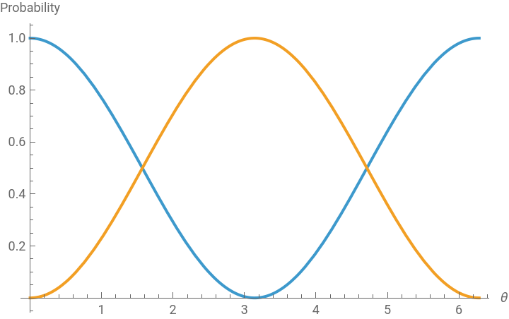


This wavy pattern is the hallmark of quantum interference. For any interference experiment, a very natural question arises: during its evolution through the apparatus, which path did the quantum system take? In the double-slit experiment, this means: through which slit did the quantum system pass?
Keep in mind that such experiments have been performed with very large molecules as well. These setups are usually called matter-wave interferometers. The quantum systems in this case, often referred to as interfering particles, are so large (around 7,000 atoms) that it is hard to imagine “exotic” scenarios, such as the particle somehow splitting into two pieces, each piece going through a different slit and then recombining. For these large macromolecules, the quantum object has a well-defined particle identity. So, if it is a particle, one is tempted to ask again: which path did it take? was it, or else? For that purpose, let’s try to store the path information and do the experiment again.
Keep in mind that such experiments have been performed with very large molecules as well. These setups are usually called matter-wave interferometers. The quantum systems in this case, often referred to as interfering particles, are so large (around 7,000 atoms) that it is hard to imagine “exotic” scenarios, such as the particle somehow splitting into two pieces, each piece going through a different slit and then recombining. For these large macromolecules, the quantum object has a well-defined particle identity. So, if it is a particle, one is tempted to ask again: which path did it take? was it
|0〉
|1〉
Storing the path information: no interference!
Storing the path information: no interference!
To store the path information (i.e., whether the system is in the state or ), we extend our Hilbert space. Specifically, we consider a simple two-qubit system whose total Hilbert space is the tensor product of the individual qubit spaces ⊗ where ⊗ (the tensor product) means we keep track of both systems at once. The tensor product is a way of combining vector spaces (and vectors) to form a larger space. . The second qubit can represent another degree of freedom of the interfering particle itself—for example, the polarization of a photon, or the momentum state of a molecule or atom. We label the degrees of freedom of the interfering particle by the subscript 1, and those of the auxiliary system by the subscript 2. The path information will be stored in this second system. For convenience, we will refer to them as qubit-1 and qubit-2. To encode the path information, we proceed as follows: we prepare qubit-2 in the initial state . If qubit-1 is in the state , qubit-2 remains in ; if qubit-1 is in the state we transform qubit-2 into . This can be implemented by a conditional operation known as the controlled-NOT (CNOT) gate in quantum computation.
|0〉
|1〉
ℋ
1
ℋ
2
|0〉
|0〉
|1〉
|1〉
|1〉
CNOT is among operations that serve as universal entanglers. You designate a control qubit and a target qubit: the CNOT gate checks whether the control is in 0 or 1, and then, depending on the choice, control-0 (if the control is 0) or control-1 (if the control is 1), it applies the NOT gate to the target qubit.
CNOT (or CX) flips the target qubit when the control qubit is in the 1 state.
In[]:=
QuantumCircuitOperator["CNOT"]"Diagram",
Out[]=
How CNOT transform 2-qubit computational basis:
Out[]=
|ψ〉 | CNOT|ψ〉 |
|00〉 | |00〉 |
|01〉 | |01〉 |
|10〉 | |11〉 |
|11〉 | |10〉 |
Now, let’s incorporate the CNOT into the previous quantum circuit:
Out[]=
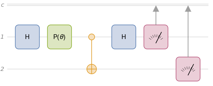
Note that it does not matter if CNOT is introduced before or after the phase shifter. As far as it is between two Hadamard gates, that is enough. Now let’s see how the system is evolved within this circuit. Given we have a composite quantum system (i.e. two qubits), then the corresponding basis elements are for qubit-1 and for qubit-2. The composite system then has dimension . Its computational basis is formed by tensoring the single-system basis states:, , , and . So the corresponding state vector is a vector of four components.
{|0〉,|1〉}
{|0〉,|1〉}
2×2=4
|00〉=⊗={1,0,0,0}
|0〉
1
|0〉
2
|01〉=⊗={0,1,0,0}
|0〉
1
|1〉
2
|10〉=⊗={0,0,1,0}
|1〉
1
|0〉
2
|11〉=⊗={0,0,0,1}
|1〉
1
|1〉
2
Calculate the system evolution through each step:
Show the states prior to measurement:
Now let’s focus on probability calculations. Since we have a composite system of two qubits, the measurement outcomes are described by joint probabilities. For example, we can consider the probability of finding qubit-1 in state 0 and qubit-2 in state 1. This joint probability can be calculated as follows:
In a similar manner, calculate the probability of observing qubit-1 in the state 1.
Did you expect this result? In other words, the interference pattern disappears! Note that the above calculations are exactly equivalent to the following scenario: given the circuit after the path information has been stored, we perform a measurement only on qubit-1 and ignore qubit-2.
Calculate the probabilities associated with the measurement outcomes of the above circuit:
In any case, even when we look at the joint probabilities (i.e., the combined statistics of qubit-1 and qubit-2), no interference pattern appears.
So when the path information is stored, even if we do not read it (as in the scenario where we do not measure qubit-2), the interference pattern disappears. It appears that the interference pattern and the path information are complementary: when path information is available, the interference pattern vanishes; when no path information is stored, the interference pattern is observed.
According to Bohr’s interpretation, the first scenario (without the CNOT gate) is a single, indivisible phenomenon that cannot be decomposed into smaller, independent parts. In this context, a question such as “which path did the particle take?” has no meaning. If we want to obtain path information, we can introduce a CNOT operation, but then the entire experimental setup becomes a different phenomenon, fundamentally distinct from the original case—and again, it must be treated as an indivisible whole. Naturally, we should expect different results in this new scenario. These two setups cannot be realized simultaneously; they represent complementary phenomena.
Erasing path information: interference
Erasing path information: interference
Compute normalized eigenvectors:
Calculate eigenvalues:
In order to measure in the Pauli-X basis, one can introduce a Hadamard gate before measuring the qubit-2 in the computational basis. It is similar to passing the second quantum system through a beam-splitter in the case of photonic system.
Construct the quantum circuit:
Calculate the system evolution through each step:
Show the states prior to measurement:
Like the previous case, calculate probabilities:
At first glance, it may seem that we have recovered an interference pattern, since the result depends on θ. However, if you look more closely, you will notice that the above expression is simply one half of what we obtained in the earlier interference case.
In a similar manner, calculate the probability of observing qubit-1 in the state 1:
You might be disappointed, because this is not the result we were hoping for: we did not recover the interference pattern for qubit-1. But if you think more carefully, this is exactly what we should expect. The only operations we performed were on qubit-2. In other words, special relativity tells us that we cannot influence one system superluminally (faster than light) by manipulating another, spatially separated system. We should not expect any change in the statistics of qubit-1 by doing whatever we like to qubit-2. If this were possible, the consequences would be dramatic. Suppose, for the sake of argument, that it were possible to change the statistics of qubit-1 by acting on qubit-2. Imagine we apply our operation on qubit-2 after qubit-1 has already been measured. Then the statistics of qubit-1 would correspond to an event in the past. Do we really expect to be able to change the past by doing something in the future? Of course not. This kind of apparent tension between quantum mechanics and causality is at the heart of what Wheeler called a delayed-choice experiment. But let us set this aside and return to the quantum eraser idea, examining carefully what we actually did and whether any interference pattern was, in fact, recovered.
Instead of looking at individual statistics (also called marginal probabilities), let’s focus on joint probabilities. For example, what is the probability of observing qubit-1 in state 0 and qubit-2 in state 0?
Calculate the probability of observing qubit-1 in state 0 and qubit-2 in state 1:
Calculate the probability of observing qubit-1 in state 1 and qubit-2 in state 0:
Calculate the probability of observing qubit-1 in state 1 and qubit-2 in state 1:
In other words, when we look at the joint probabilities (i.e., the combined outcomes of qubit-1 and qubit-2), we succeed in recovering the interference pattern.
I’d like to remind the reader that the interference pattern is recovered only at the level of joint probabilities. For the marginal probabilities (the statistics of qubit-1 alone), the interference pattern is not recovered. This is exactly what we should expect from Einstein’s relativity: we cannot influence the statistics of one system by performing operations on another spatially separated system.
Another interesting fact is that the path information can be erased only partially. This can be achieved by applying a rotation gate about the y-axis, with a chosen angle ϕ, instead of a Hadamard gate, on qubit-2. Therefore, depending on the angle ϕ, the erasure of which-path information can vary continuously from none (no erasure) to complete (full erasure).
Construct a quantum circuit for variable path erasure:
Calculate the corresponding measurement probabilities:
Concluding remarks
Concluding remarks
A quantum system can exhibit contrasting features under different experimental conditions. In some setups it behaves like a particle, while in others it behaves like a wave. In the wave-like case, the quantum system is delocalized and produces an interference pattern, which seems to contradict the particle picture. The situation becomes even more subtle when we consider experiments performed one particle at a time: individual particles are detected one by one at the detector, yet the accumulated statistics reveal an interference pattern.
Quantum erasure provides a clever way to rearrange the marginal probabilities so that the corresponding joint probabilities once again display an interference pattern. The key point is that the interference pattern in the joint probabilities is recovered only when the which-path information is erased. However, these complementary phenomena occur in mutually exclusive experimental contexts, and their associated probabilities are computed under mutually exclusive conditions. The change in conditions, characterized by a transformation of the quantum state, arises from local interactions. The marginal probabilities, which describe the statistics of individual particle detections, cannot be altered merely by erasing the path information.
Quantum erasure provides a clever way to rearrange the marginal probabilities so that the corresponding joint probabilities once again display an interference pattern. The key point is that the interference pattern in the joint probabilities is recovered only when the which-path information is erased. However, these complementary phenomena occur in mutually exclusive experimental contexts, and their associated probabilities are computed under mutually exclusive conditions. The change in conditions, characterized by a transformation of the quantum state, arises from local interactions. The marginal probabilities, which describe the statistics of individual particle detections, cannot be altered merely by erasing the path information.
Initialization
Initialization
Install Wolfram quantum framework:
References
References
Some selected references on this topic:
N.Bohr (1935), Can quantum-mechanical description of physical reality be considered complete?
N.Bohr (1949) Discussions with Einstein on Epistemological Problems in Atomic Physics
Wootters, Zurek (1979), Complementarity in the double-slit experiment: Quantum nonseparability and a quantitative statement of Bohr’s principle
J. A. Wheeler, (1979), Law Without Law
Bartell (1980), Complementarity in the double-slit experiment: On simple realizable systems for observing intermediate particle-wave behavior
M.O. Scully and K. Druhl (1982), Quantum eraser: A proposed photon correlation experiment concerning observation and “delayed choice” in quantum mechanics
T. Hellmuth, H. Walther, A. Zajonc, and W. Schleich (1987(, Delayed-choice experiments in quantum interference
M .O. Scully, B. G. Englert, and H. Walther (1991), Quantum optical tests of Complementarity
T. J. Herzog et al (1995), Complementarity and the Quantum Eraser
C. C. Gerry (1996), Complementarity and quantum erasure with dispersive atom-field interactions
U. Mohrhoff (1996), Restoration of interference and the fallacy of delayed choice: Concerning an experiment proposed by Englert, Scully, and Walther
B. G. Englert, M. O. Scully, and H. Walther (1998), Quantum erasure in double-slit interferometers with which-way detectors
U. Mohrhoff (1999), Objectivity, retrocausation, and the experiment of Englert, Scully, and Walther
Durr, Rempe (2000), Complementarity and quantum erasure in an atom interferometer
C. Elitzur, S. Dolev (2002), Time-Reversed EPR and the Choice of Histories in Quantum Mechanics
Bramon and G. Garbarino (2003), Quantum marking and quantum erasure for neutral kaons
Y. Aharonov and M. S. Zubairy (2005), Time and the Quantum: Erasing the Past and Impacting the Future
Jacques et al (2006), Experimental realization of Wheeler’s delayed-choice Gedanken Experiment
T. Norsen (2006), Comment on “Experimental realization of Wheeler’s delayed-choice GedankenExperiment”
J. Hiley and R. E. Callaghan (2006), Delayed Choice Experiments and the Bohm Approach.
M. Bahrami and A. Shafiee (2009), Postponing the Past: An Operational Analysis of Delayed-Choice Experiments
CITE THIS NOTEBOOK
CITE THIS NOTEBOOK
Quantum interference loss via path encoding and recovery by quantum erasure
by Mohammad Bahrami
Wolfram Community, STAFF PICKS, November 18, 2025
https://community.wolfram.com/groups/-/m/t/3577822
by Mohammad Bahrami
Wolfram Community, STAFF PICKS, November 18, 2025
https://community.wolfram.com/groups/-/m/t/3577822