We model a social network as a complete weighted graph, where pairs of vertices repeatedly play two-player games against each other. The weight of each edge act as a proxy for the strength of the relationship between its vertices and is updated each round according to the outcome of that pair’s game. Varying parameters such as the number of players, method by which payoffs are combined, and weight function, we track a set of statistical metrics on the resulting edge weights. We also allow players to adapt their strategies over time—and take on various social temperaments—and investigate how these dynamics vary with the nature of the games being played.
Motivation
Motivation
Consider a group of people: they don’t know each other and have no shared history. What happens when they are suddenly placed in a situation where they must repeatedly interact with each other? How do the relationships between them evolve? Do they go their separate ways, build strong connections, or form cliques? Do certain individuals isolate themselves? (I’ll cheekily highlight the parallel between what I’ve just proposed and the social premise of the WSRI program where this project was produced.)
We can model this with a complete graph of vertices, where is the number of people in our group. Every vertex is connected to every other vertex by an edge which represents their relationship. If we assign a weight to each edge (say, between 0 and 1) to describe the strength of this relationship, we can initialize our graph with weights of 0.5 to say that our players are essentially starting from a “blank slate.”
n
n
An example with :
n5
Out[]=
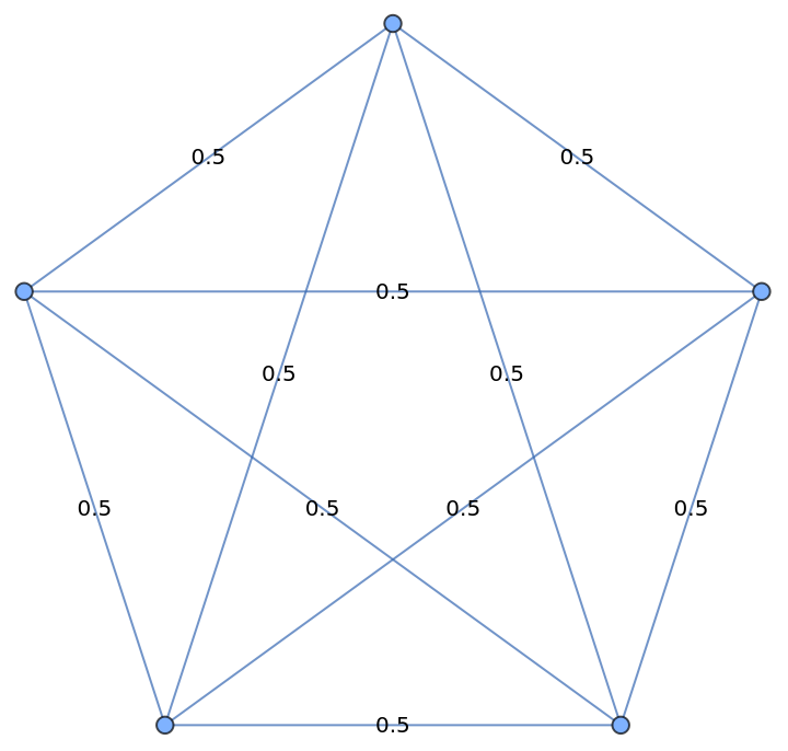
Then we can allow our vertices to play games with each other to simulate the natural interactions that occur between members of a social network. If a pair of vertices achieves some “good outcome” (a more rigorous definition of this will be established later), then we increase the weight of the edge connecting them. After some repetition, we can check the weight of the edges again to see how our group has evolved over time.
An Example
An Example
Let’s begin with a simple example to better understand how our setup works. Take our earlier graph with 5 players. Every round, the vertices—or players—will participate in a game with each other.
A Brief Introduction to Games
A Brief Introduction to Games
So what is a game? For those unfamiliar with game theory, in this project we use a basic way of defining two-player games. For a given game we have the following properties:
◼
Players: the agents (vertices) participating
◼
Strategies: the actions the players can take in a round
◼
Outcome: given the chosen strategies of all the players, the result of the game
◼
Payoff: given the outcome, a measure of what each player “gets” (one can consider this a kind of utility)
◼
This can be represented in a payoff matrix. For example, a simple instance of a game is Matching Sides, where the players choose heads or tails and both obtain payoff 1 should they choose the same side, and 0 otherwise. We can represent the possible payoffs of this game in a matrix, where cell represents the outcome where player 1 plays and player 2 plays . Each cell contains an ordered pair, where the first element is the player 1’s payoff under that outcome and the second element is that of player 2.
ij
i
j
Out[]=
|

The Prisoner’s Dilemma
The Prisoner’s Dilemma
One of the most famous games in game theory—and the one we’ll use for our example here—is the Prisoner’s Dilemma. It’s defined as the following:
The two players in the game are criminals who have been arrested by the police. They’re interrogated separately and simultaneously, so they may not collaborate. They’re given two options: to confess to the crime they presumably committed together or to cooperate (stay silent). If neither confesses, they’ll both go to prison for one year. If one confesses and the other stays silent, the confessor will go free and the other will go to prison for five years. If both confess, they’ll both go to prison for three years. The way that payoff is defined is somewhat arbitrary, so to keep things simple we’ll say that the payoff of each player is (negative) the number of years they’ll go to prison. Then we can use the following payoff matrix to understand the game:
Out[]=
|
Although this is mostly irrelevant for our project, notice that a rational player would always choose to confess: regardless of which choice their partner-in-crime makes, they’ll always receive a higher payoff from confessing; however this is obviously not the “optimal” outcome (in the sense that {Cooperate, Cooperate} in fact has the highest total payoff). It would be a rather boring game if each player were to simply play rationally and choose the same strategy each time, so instead we’ll define our players’ strategies randomly. That is, each player is assigned a (personal) random probability of confessing (and hence probability of cooperating), and each round they make a random weighted draw based on this probability. In more technical terms we define a “strategy matrix,” where element is player ’s probability of playing :
p
1-p
ij
i
j
Out[]//MatrixForm=
3 7 | 4 7 |
69 142 | 73 142 |
71 113 | 42 113 |
19 110 | 91 110 |
75 169 | 94 169 |
We now have what we need to try running our game. We’ll save some of the technical specifications of how we define a good outcome of a game and how the edge weights are updated for later and simply try simulating the Prisoner’s Dilemma with our five players. After one round:
Out[]=
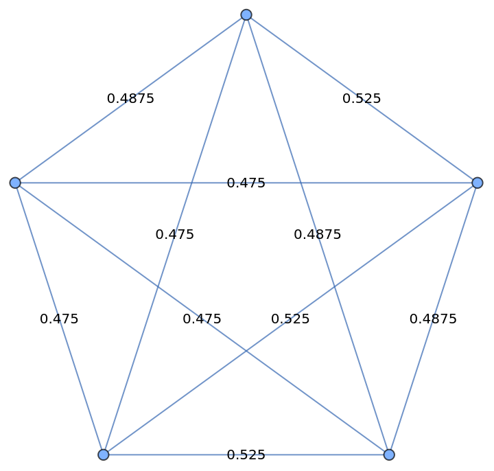
Notice that some of the edge weights increased and others decreased, but the change is relatively minimal. What happens if we repeat this over, say, 100 rounds? To visualize the evolution of our graph we’ll color edges with higher weights with higher opacity.
Out[]=
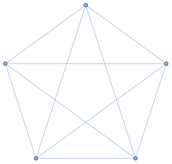
We see that some pairings of players emerge with higher weights, while others seem to fade away—we can think of this, in terms of our social network, as the strengthening or weakening of relationships. This naturally leads us to the question: do these weights “stabilize” in some sort of way, as one could imagine a network might as members form judgments on each other? Can we measure this and determine with a threshold when our graph has reached a stable state?
Stability
Stability
One simple measure of stability is total change. In a given round, we sum the absolute values of weight changes from the last round for each edge and declare our graph “stable” when this index falls below a threshold. Let’s take a look at our stability index over 100 rounds:
Out[]=
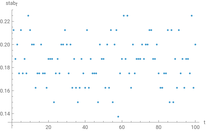
Unfortunately it seems like this index doesn’t follow a distinct downward trend at this scale and hence we can’t assign a meaningful threshold to detect a stable state. Checking the last 100 stability indices from a 1000-round run:
Out[]=
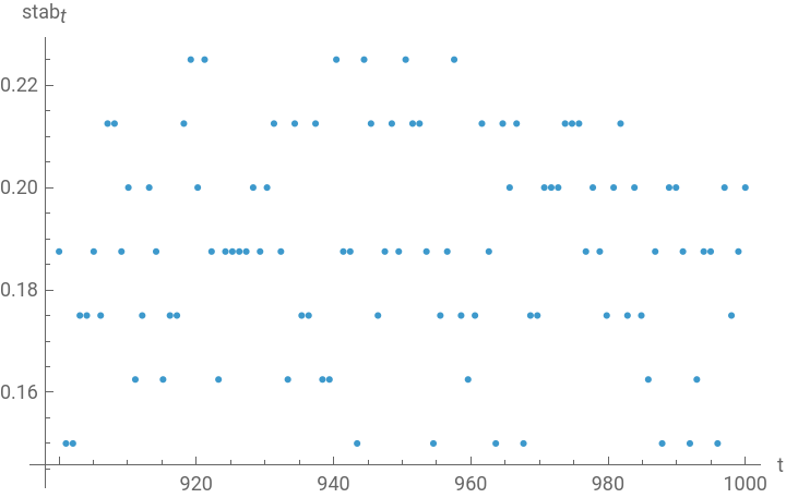
We get similar results—the stability index doesn’t decrease, even towards the end of a longer run. We’ll set this aside for now and attempt to return to it later once we’ve properly defined a more generalized description of our simulation, which we’ll do now.
The Setup
The Setup
We start with a complete graph of vertices. Each vertex models one agent or player, and each edge represents a symmetric game between players (or vertices) and . For now we assign a weight of 0.5 to every —the weight of an edge, , represents the degree of successful cooperation between the two agents it connects.
n
{i,j}
G
i
j
edge
w∈[0,1]
Each round we simulate every edge playing once. Our goal is to adjust the weight of the edge proportional to how well the agents cooperated. For a given edge we follow these steps:
G
{i,j}
1
.Select a strategy for each agent, simulate the game, and find the payoffs
2
.Generate a normalized collaborative index
2
.1
.We first apply a function to find a collective payoff —the base example being simply addition:
π
π(i,j)+
π
i
π
j
3
.Adjust the weight of the edge
Variations
Variations
Now that we have a more technical understanding of the procedures for our simulation, we can explore some different parameters. So far we’ve been mostly relying on visual examination and heuristics; let’s explore some metrics so that we can observe more concretely how these parameters affect our graph.
Graph Metrics
Graph Metrics
One rather intuitive set of metrics we may want to explore is the standard set of statistical measures on the edge weights on our graph. On the final graph we obtain after a simulation, we can collect all the edge weights and compute their mean, median, standard deviation, and distribution. This gives us a healthy, if somewhat general, idea of how our graph has evolved.
A more specialized metric we can use is the global clustering coefficient on weighted graphs proposed by Opsahl and Panzarasa [1], using the method of arithmetic means (a technical definition can be found here).
Weight Function
Weight Function
Recall the monotonic, bounded function we used to adjust the weight of our edges. In our original example we used a naive “constant addition” function, where the rate of change for the weights was independent of the current weight of the edge. But we can introduce some other options:
For the latter two functions (the logistic function and the integral of the negative absolute value function, respectively), notice that weights become less volatile as they get closer to the extremes. Repeating our example with the logistic function as our weight function, for example:
We can further investigate the properties of these weight functions by looking at the metrics we defined earlier.
Interestingly, with a more complex graph, we get very similar results between the three methods of weight adjustment! Notice also that almost all of the edges end up with a very low weight, with higher weights uniformly distributed for the most part throughout the rest of the range (except for the top range, which has slightly more edges). This indicates that there’s probably some sort of negative drift.
Cooperation Index
Cooperation Index
◼
Substituting the sum in our original example for a geometric mean and running for 50 periods:
◼
And the same setup with a harmonic mean:
With our higher count of vertices the patterns become a bit more complex, but we can see quite clearly that the arithmetic and geometric means isolate certain edges much more so than the harmonic mean, which maintains a mostly stable and complete graph. In particular, the geometric mean finds fewer connected, strong vertices—we can think of this as the network containing a few very social members while others remain isolated—while the arithmetic mean preserves more relationships overall.
Now that we’re seeing evolutions that at least appear to converge somewhat, let’s revisit the stability index we defined earlier. Generating stability indices for our three methods of determining collective payoff (again checking the last 100 of 1000 rounds):
Still, our stability index seems to remain fairly consistent up to 1000 rounds (possibly due to the way we’ve defined it)—so let’s again look at the metrics we defined earlier:
Notably, none of our methods are “unbiased”: the sum and geometric mean push weights down to 0, revealing a select few edges that persist, while the harmonic mean tends to increase edge weights. The global clustering coefficients then make sense—the harmonic mean generates a graph which remains mostly complete. Even with a complex graph, the way information about payoffs is integrated makes a significant difference on the characteristics of our graph.
Before we proceed, let’s establish a set of default parameters to work off of for the rest of this essay: unless otherwise specified, we’ll assume that each simulation uses a graph with 20 players, takes the sum as the cooperative index, updates weights with the logistic function, and iterates for 100 rounds.
Temperament
Temperament
The Selfish Player
The Selfish Player
We begin with the naive case: each player only cares about their own payoff. Each round, they consider the strategies they played and the payoffs obtained from those strategies, increasing their probability of playing strategies that earned higher payoffs next round.
Let’s see how this new protocol compares against our old settings:
It’s clear that (at least our current version of) evolving strategies destroys almost all relationships within our network. If we think back to the definition of our game, it’s pretty easy to see why: I mentioned as an aside in the beginning that in the Prisoner’s Dilemma, if a player plays only to maximize their own payoff, they will always choose to confess; however {Confess, Confess} actually yields the lowest total payoff of the four possible outcomes. Thinking about how our strategy adjustment works, regardless of which strategy a player’s partner played, they’ll always get a higher payoff by confessing and hence increase the probability of confessing the next round. As the simulation goes on, more players shift their strategies to confessing and relationships break down from the low payoffs of the outcome {Confess, Confess}.
The Altruist, the Masochist, and the Sadist
The Altruist, the Masochist, and the Sadist
(Technically in the social sciences this way of measuring how an individual attributes value to their own and others’ welfare is called social value orientation, or SVO.)
Other Games
Other Games
Fortunately, life is not the Prisoner’s Dilemma (it would be quite sad if we were all being interrogated by the police 100 days in a row). So let’s explore some other games:
◼
Battle of the Sexes: a classic game where, traditionally, a husband and wife disagree about their plans for the evening. The husband wants to go to a boxing match, and the wife wants to attend the ballet. Both would prefer their activity of choice, but they care more that they end up at the same activity.
◼
Chicken: two high school students are driving towards each other. They’re in a game of chicken—if one swerves and the other keeps driving, the person who swerved loses some points for being the chicken; nothing happens if both swerve; and if they drive into each other, they both die.
Rather than collapsing to extreme edge weights, these edges seem to mostly fluctuate, and the graph maintains a healthy distribution of edges of the full range of weights (we can see this more clearly in the histogram).
Games with More Strategies
Games with More Strategies
◼
Rock-paper-scissors
◼
Matching colors: the same premise as Matching Sides, but there are three colors and the players are trying to select the same one.
◼
We can also randomly generate games. Here’s an example with 5 strategies for each player, with maximum payoff 10:
(Find the results for rock-paper-scissors and the random 5x5 game in the Appendix.)
With rock-paper-scissors the results are predictably rather boring since the total payoff of each outcome is always 0, so the weights never shift; we find our more interesting results with Matching Colors. We can apply similar reasoning as we did previously to consider why certain temperaments create distinct edge weight distributions in these specific games—an effort we’ll leave as an exercise for the interested reader—but instead we’ll try to make some general observations about which types of games tend to create which kinds of results in the following section.
Unfortunately there are far too many parameters in our simulation for us to perform a comprehensive analysis of all the different combinations, but here you can make up your own 2x2 game and set each parameter as you like to see how your graph evolves!
Concluding Remarks
Concluding Remarks
Throughout this exploration we’ve defined several variations on the basic premise of a social network evolving by way of its members playing games with each other. Most notably:
◼
Various methods of combining payoff between players (arithmetic, geometric, and harmonic mean) produce drastically different distributions of edge weights, where each method pushes the edge weights to an extreme.
◼
With the Prisoner’s Dilemma, a game where there’s an “objectively good” strategy, allowing players to adapt their strategies to payoffs and assigning a selfish temperament leads to the breakdown of relationships.
◼
A brief investigation of other games shows that games where the “correct” choice is less obvious and which involve some sort of random coordination (such as Battle of the Sexes and Matching Colors) are less responsive to evolving strategies but develop some interesting patterns.
◼
For instance, Battle of the Sexes sees higher mean edge weights when player temperaments live in the first quadrant.
Limitations
Limitations
Future Work
Future Work
We see some clear ways in which this work can be expanded upon:
◼
This essay only addresses two-player games, but hypergraphs can be used to model games with more players
◼
Continuous games, where players select strategies from a continuous probability distribution
◼
More “intelligent” players that adjust their strategies to account for future payoff or “goodwill” between players
◼
Players that play different strategies against each partner, or players with different temperaments within the same network and how they interact
Acknowledgements
Acknowledgements
Many thanks to my mentor Zsombor Méder—this project wouldn’t have happened without his guidance, input, and suggestions, and I’m grateful for the generous time and support he’s given me throughout the WSRI program. I also wish to acknowledge Stephen Wolfram for the initial idea which set this project in motion, and my deepest thanks to Rico Chung for kindly reviewing and proofreading this work.
References
References
1
.T. Opsahl and P. Panzarasa (2009), “Clustering in Weighted Networks,” Social Networks 31(2). https://toreopsahl.com/wp-content/uploads/2009/03/clustering.pdf.
AI Disclosure
AI Disclosure
We used Claude Opus 4.8 in this project for the following:
◼
Debugging code
◼
Proofreading prose
◼
Sanity checks
◼
Formatting interactive elements
All code and written content was reviewed, understood, and approved by the author.
Appendix
Appendix
Functions
Functions
Cite This Notebook
Cite This Notebook
"On Games and Graphs"
by Mia Zhao
Wolfram Community, 17 July 2026
by Mia Zhao
Wolfram Community, 17 July 2026