Out[]=

Visualize the configuration. I use Canvas function to sketch the diagram
In[]:=
Canvas[]
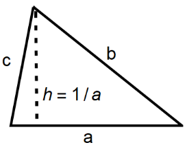
The length of the altitude is from that . The altitude divides the triangle into two parts and the foot divides a into two sections. Using Pythagorean theorem, let’s solve for a w.r.t b and c.
Area·h·a
1
2
In[]:=
Uniona/.Solve
(b^2-1/a^2)
+(c^2-1/a^2)
a,a^2Out[]=
+-2++2
2
b
2
c
-1+
,2
b
2
c
2
b
2
c
-1+
2
b
2
c
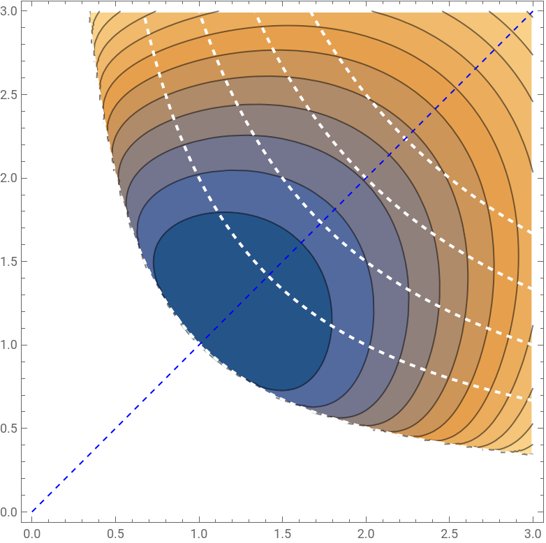
Also we know , thus . Our target function can be visualized with contour plot. White dashed lines are contours for .
Areab·c·sin(A)
1
2
csc(A)b·c
b·c
In[]:=
ContourPlot+-2
2
b
2
c
-1+
+b*c,{b,0,3},{c,0,3},Contours12,MeshFunctions{#1*#2&},Mesh{{1.01,2,3,4,5}},MeshStyle{White,Thick,Dashed},Epilog{Dashed,Blue,Line[{{0,0},{3,3}}]},BoundaryStyleDirective[White,Thick]2
b
2
c
Out[]=
Now we can try to find minimum value
In[]:=
Minimize+-2
2
b
2
c
-1+
+b*c,b>0,c>0,b*c>1,{b,c}//FullSimplify2
b
2
c
Out[]=
,c
5
,b3
1/4
5
3
1/4
5
There is another way to find the minimum. If we interchange b and c , the target function is unchanged. Therefore we can use educated guess to find the minimum along .
bc
In[]:=
PlotEvaluate+-2
2
b
2
c
-1+
+b*c/.bc,{c,1,2}2
b
2
c
Out[]=
Now we have a single valued function
In[]:=
expr=Evaluate+-2
2
b
2
c
-1+
+b*c/.bc//FullSimplify2
b
2
c
Out[]=
3-2
2
c
-1+
4
c
We can also find the global minimum by
In[]:=
Minimize[{expr,c>0},c]
Out[]=
5
,c3
1/4
5