Exploring the effects of causal graph dimension variations in null geodesics
by Joana Teixeira
University College London
by Joana Teixeira
University College London
The purpose of this project is to explore the effects of local dimension variations on the propagation of null geodesics in causal graphs . We choose a particular approach to tackle this issue, which is by no means exhaustive. We focus on causal graphs obtained by sprinkling rather than by the evolution of a Wolfram Model rule, which have the simplifying feature of having coordinates associated with each vertex. The local dimension of the graph is perturbed at a point by adding edges to it , and we explore how the change in local dimensions depends on these new edges . In order to investigate how the dimension perturbations affect the null geodesics, we look at the shape of the boundary of future light cones (the horismos). In particular, we look at how the dimension perturbation affects the mean position and mean deviation of projections of the horismos into slices of constant affine parameter (the causal layers). We measure the correlations between these changes and the dimension perturbation and found that there was no obvious correlation between the them. We suggest some explanatory hypotheses for these results, and discuss how these analyses may be performed in a coordinate-independent fashion for the case of causal graphs produced by Wolfram model evolution.
Introduction
Introduction
Motivation and outline
Motivation and outline
In order to explore whether Wolfram Models [1] describe the physical world, it is important to look for observables where the discreteness of spacetime would leave an imprint. One particular feature of having a discrete space/spacetime, such as those produced by the evolution of Wolfram Model rules, is that the local dimensions of such spaces are not the same everywhere, and don’t necessarily correspond to the global dimension. So if space/spacetime are indeed discrete, it is expectable that there are small local dimension perturbations. But the main question is: could these have a measurable effects in any experiments we might devise in the future? One hypothesis is that dimension perturbations might have a lensing-like effect, similarly to gravitational lensing observed due to curvature perturbations. The aim of this project is to perform some initial investigations on whether this is the case, by looking for changes in the properties of the horismos caused by dimension change.
In order to perform the calculations used in this project, we made use of some concepts regarding casual graphs, in particular with respect to dimension estimation and perturbations and the definition of the horismos. These are described in the Key concepts subsection below. The specific methodology used for the project is described in the Methodology section. The main calculations and results are presented in the Key Results section, which is followed by some concluding remarks, including some suggestions of future explorations, in the Conclusions section. For clarity, all the functions written for this project are grouped as an appendix, at the end of the notebook, in the Appendix 1- Necessary Functions section. Some ideas of other sprinklings on which to run the analysis are given in Appendix 2.
In order to perform the calculations used in this project, we made use of some concepts regarding casual graphs, in particular with respect to dimension estimation and perturbations and the definition of the horismos. These are described in the Key concepts subsection below. The specific methodology used for the project is described in the Methodology section. The main calculations and results are presented in the Key Results section, which is followed by some concluding remarks, including some suggestions of future explorations, in the Conclusions section. For clarity, all the functions written for this project are grouped as an appendix, at the end of the notebook, in the Appendix 1- Necessary Functions section. Some ideas of other sprinklings on which to run the analysis are given in Appendix 2.
Key concepts
Key concepts
Sprinkling
Sprinkling
A causal graph is a directed acyclic graph, i.e. a graph where the edges have a direction and where no closed cycles occur. It is in essence a collection of causal relations (edges) between elements (vertices). As such, in theory it is not difficult to produce a general causal graph. However, the causal graphs we are interested in are those which can be thought of as a discretisation of spacetime, i.e. graphs whose continuum limit would approach a certain continuous spacetime. The topic of how to produce such graphs has been studied by several people, e.g. in the context of Causal Set Theory, and one of the techniques which is used for this is sprinkling (see e.g. [2] for some discussion on this). At a high level, sprinkling consists of randomly picking some points from an underlying spacetime, and using the causal relations of the points in the underlying spacetime to define the edges in the resulting discrete graph (for details see discussions in e.g. [2]). These sprinklings must follow a specified probability distribution: in particular, the vertices must be uniformly distributed in the spacetime, in such a way that the number of points in a certain volume of spacetime is proportional to that volume.
Luckily, functions have already been written in Wolfram Language to produce such sprinklings very easily. For example, here we create a causal graph by sprinkling points onto a Minkowski spacetime:
Luckily, functions have already been written in Wolfram Language to produce such sprinklings very easily. For example, here we create a causal graph by sprinkling points onto a Minkowski spacetime:
In[]:=
ClearAll[exampleSprinkling,exampleCausalGraph]exampleSprinkling=ResourceFunction["FlatSpacetimeSprinkling"][2,200];exampleCausalGraph=exampleSprinkling["CausalGraph"];
The time coordinate of the vertices of graphs resulting from the sprinkling resource functions is their final coordinate, and it decreases as time increases (i.e. time moves downwards along the graphs, with events of higher t corresponding to earlier events).
Once we have this graph, we can use all the Wolfram Language graph functionality on it. For example, given a certain vertex, we can find the equivalent of that vertex’ past (or future) light cone by finding all the vertices which have a directed path to (or from) that vertex. Below we exemplify this; we select an exampleVertex with time coordinate larger than 0.6 for visualization purposes:
Once we have this graph, we can use all the Wolfram Language graph functionality on it. For example, given a certain vertex, we can find the equivalent of that vertex’ past (or future) light cone by finding all the vertices which have a directed path to (or from) that vertex. Below we exemplify this; we select an exampleVertex with time coordinate larger than 0.6 for visualization purposes:
Out[]=
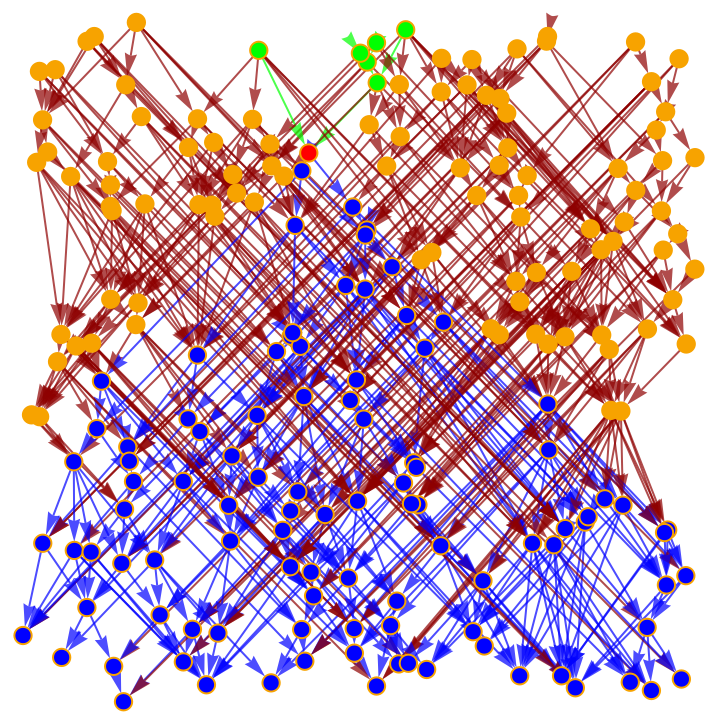
Horismos
Horismos
Now that we have a discrete spacetime and can find past and future light cones of events (here described by vertices), we are in a position to define the horismos of a vertex.
In continuous spacetime, the horismos is the boundary of the future light cone, i.e. it is the set of all points in the future light cone which are light-like separated from the origin event. While this is an obvious thing to calculate in continuous spacetime (light-like separated points are points v1 and v2 whose position difference v2-v1 is a null vector, i.e. has norm zero), this is not as straightforward in the case of discrete spacetimes. We present two methods for finding the horismos of a vertex, one using the point coordinates (very handy for causal sets built from sprinkling) and one using combinatorics.
In continuous spacetime, the horismos is the boundary of the future light cone, i.e. it is the set of all points in the future light cone which are light-like separated from the origin event. While this is an obvious thing to calculate in continuous spacetime (light-like separated points are points v1 and v2 whose position difference v2-v1 is a null vector, i.e. has norm zero), this is not as straightforward in the case of discrete spacetimes. We present two methods for finding the horismos of a vertex, one using the point coordinates (very handy for causal sets built from sprinkling) and one using combinatorics.
1) Coordinate - based definition
Using the coordinates, we can simply calculate the norm of the displacement vector between the origin vertex and all points in its causal future and check which ones are approximately null. Due to the fact that spacetime is now discrete, the probability that the norm will be exactly zero is vanishingly small; so we need to set some tolerance for the norm, epsilon, below which we consider the vector to be null. The choice of epsilon is rather arbitrary, but a sensible choice is for it to be proportional to the spatial density of points (see Necessary Functions section). So the horismos of the exampleVertex can be easily found, and is shown (in blue) on top of the future light cone (in green) below .
Using the coordinates, we can simply calculate the norm of the displacement vector between the origin vertex and all points in its causal future and check which ones are approximately null. Due to the fact that spacetime is now discrete, the probability that the norm will be exactly zero is vanishingly small; so we need to set some tolerance for the norm, epsilon, below which we consider the vector to be null. The choice of epsilon is rather arbitrary, but a sensible choice is for it to be proportional to the spatial density of points (see Necessary Functions section). So the horismos of the exampleVertex can be easily found, and is shown (in blue) on top of the future light cone (in green) below .
Out[]=
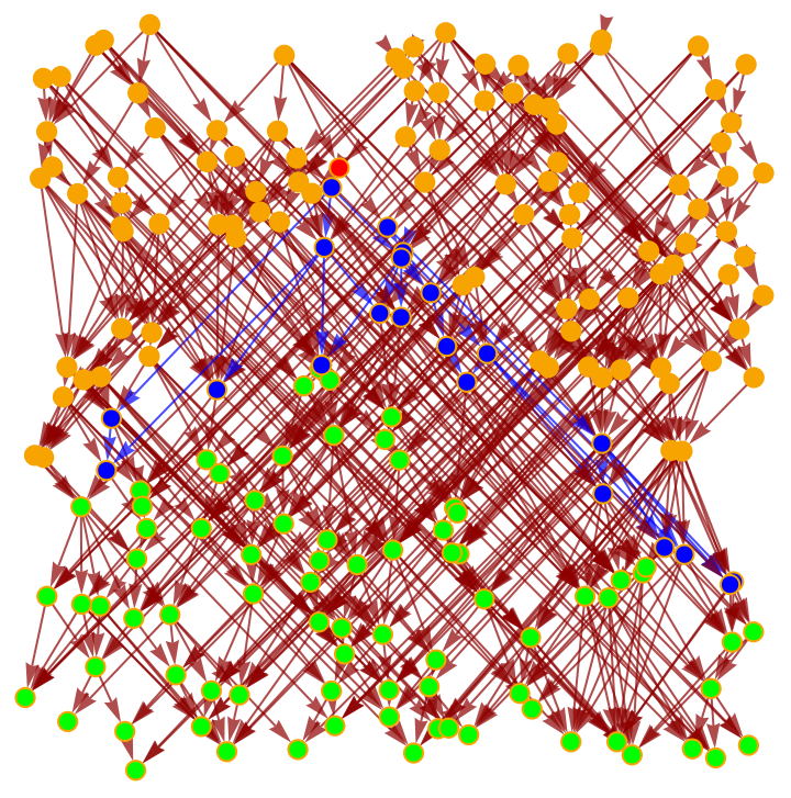
In a general causal graph without coordinate information, we need an alternative definition of lightlike separated events. We explored two ways of doing this, motivated by the (yet unproven, but reasonable) assumption that the geodesics in these discrete graphs behave similarly to those in the continuum spacetimes into which they were sprinkled. In a Lorentzian manifold, a future pointing null geodesic between two nearby points is a geodesic which minimizes proper time (which is not necessarily the case for timelike curves) and, for certain assumptions on the underlying manifold, there will be a unique path of minimal length between them [3]. So one hypothesis is that we can use the number of paths or shortest paths between two causally related vertices to determine whether they are time like or light like separated.
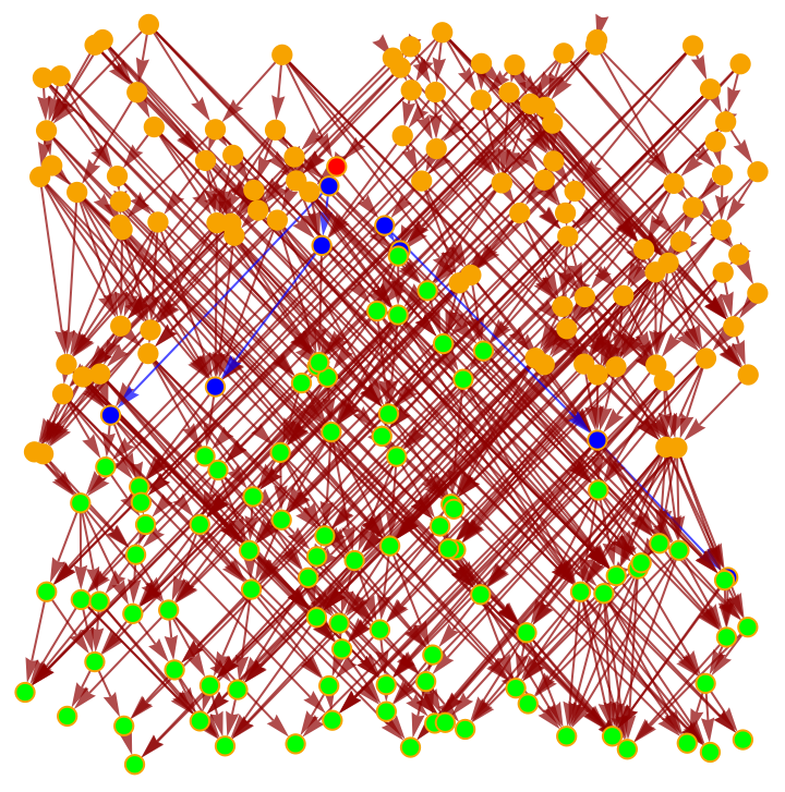
We attempted to do this is two ways: using the more theoretically motivated idea of finding points with a single shortest path to the origin vertex, and the more empirically intuitive idea of finding points with a single path to the origin vertex. So, the combinatorics horismos calculation consists of finding all the points which have a single path/ shortest path separating them from the origin vertex. Below is the same figure as above, but now with the horismos calculated using these two combinatorics definition (top: single path; bottom: single shortest path).
We attempted to do this is two ways: using the more theoretically motivated idea of finding points with a single shortest path to the origin vertex, and the more empirically intuitive idea of finding points with a single path to the origin vertex. So, the combinatorics horismos calculation consists of finding all the points which have a single path/ shortest path separating them from the origin vertex. Below is the same figure as above, but now with the horismos calculated using these two combinatorics definition (top: single path; bottom: single shortest path).
Out[]=
Out[]=
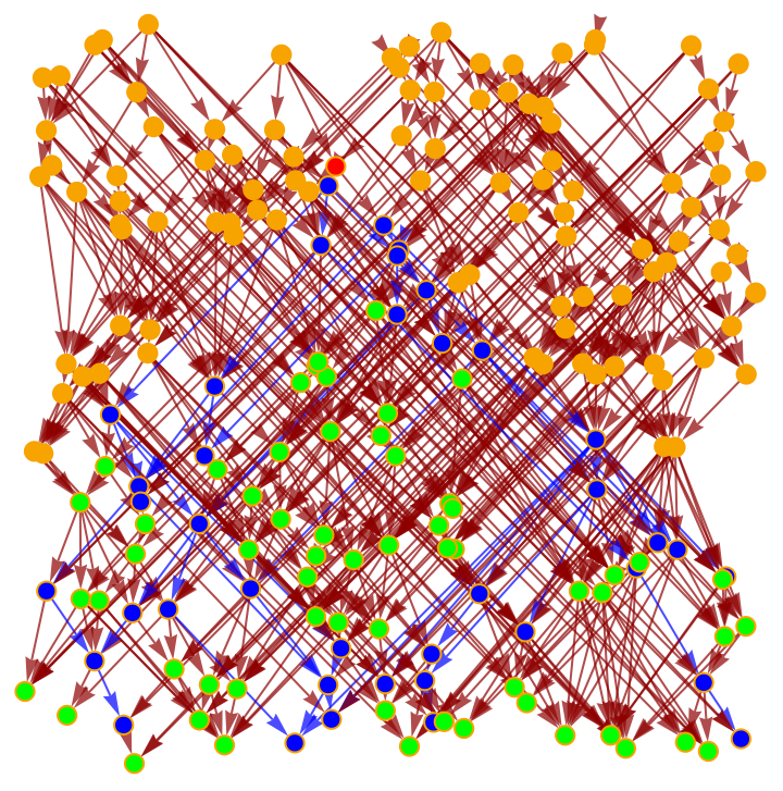
It is clear that, although the coordinate-dependent and coordinate-free definitions of the horismos are not exactly coincident for any of the two definitions. The number of vertices included in the horismos seems to be closest to the coordinate definition when using a unique shortest path. However the shape seems much more reasonable when using the unique path definition. This is something which needs to be better investigated.
Throughout this project, only the coordinate-dependent definitions of the horismos was used. However, we believe that having a combinatorics definition will be very useful once the analysis performed in this project is extended to causal sets with no coordinate information.
Throughout this project, only the coordinate-dependent definitions of the horismos was used. However, we believe that having a combinatorics definition will be very useful once the analysis performed in this project is extended to causal sets with no coordinate information.
Dimension estimation
Dimension estimation
The notion of dimension estimation for discrete spaces/ spacetimes has been an object of research for many years. One field where this is particularly relevant is in Causal Set Theory. As an example, [2] explains how a set of Myrheim-Meyer estimators can be used for dimension calculations of hypergraphs and causal graphs; in [4] two different types of dimension estimates are described, namely the Minkowski dimension and a Hausdorff dimension estimator.
Taking two of these examples is enough to understand the diversity of possible estimators. For instance, the Myrheim-Meyer estimators exploit the fact that the probability of a pair of elements in an Alexandrov interval (i.e. the diamond-like portion of spacetime corresponding to the intersection of the past light cone of one point and the future light cone of another) being causally related is proportional to the volume of this interval, which itself is a function of dimension. Using this, it it possible to relate the dimension of a spacetime to the expectation value of the number of causal relations in an Alexandrov interval (please see [2] for a detailed derivation). The Hausdorff estimator, on the other hand, is based on how a volume should increase with radius in different dimensions (e.g. we know that in 2D Euclidian space the volume grows as V~and in 3D as V~), and so this method estimates the dimension of spacetime by measuring the leading power contribution (other terms are related to e.g. curvature, which is not relevant for the purpose of this project) to how the volume of that space grows with increasing radius.
Given the variety of possible dimension estimators, it is important to understand the one chosen for this project, as well as the rationale for it. In this project we use a Wolfram Hausdorff Dimension estimator, which is a discrete approximation of the Hausdorff dimension. This estimation algorithm has already been implemented in the Wolfram Language, and is available in the Resource Function as WolframHausorffDimension, and it is explained in detail in its documentation page [5]. For the case of causal graphs, the radius is the number of edges from an origin vertex, and the volume is the number of vertices which are within that radius (as we’ve seen at the start of this section, in a valid sprinkling the number of points in a certain volume is proportional to that volume). Because the graph is directed, as we increase the causal radius we encompass a larger geodesic cone,and it is the volume of this cone which is used for the dimension calculation. One of the reasons which led to the choice of this estimator for the purpose of this project was the fact that it can be used as a local dimension estimator, as it is calculated at some vertex. This is very useful when studying local dimension perturbations, as we intend to do in this project.
Taking two of these examples is enough to understand the diversity of possible estimators. For instance, the Myrheim-Meyer estimators exploit the fact that the probability of a pair of elements in an Alexandrov interval (i.e. the diamond-like portion of spacetime corresponding to the intersection of the past light cone of one point and the future light cone of another) being causally related is proportional to the volume of this interval, which itself is a function of dimension. Using this, it it possible to relate the dimension of a spacetime to the expectation value of the number of causal relations in an Alexandrov interval (please see [2] for a detailed derivation). The Hausdorff estimator, on the other hand, is based on how a volume should increase with radius in different dimensions (e.g. we know that in 2D Euclidian space the volume grows as V~
2
r
3
r
Given the variety of possible dimension estimators, it is important to understand the one chosen for this project, as well as the rationale for it. In this project we use a Wolfram Hausdorff Dimension estimator, which is a discrete approximation of the Hausdorff dimension. This estimation algorithm has already been implemented in the Wolfram Language, and is available in the Resource Function as WolframHausorffDimension, and it is explained in detail in its documentation page [5]. For the case of causal graphs, the radius is the number of edges from an origin vertex, and the volume is the number of vertices which are within that radius (as we’ve seen at the start of this section, in a valid sprinkling the number of points in a certain volume is proportional to that volume). Because the graph is directed, as we increase the causal radius we encompass a larger geodesic cone,and it is the volume of this cone which is used for the dimension calculation. One of the reasons which led to the choice of this estimator for the purpose of this project was the fact that it can be used as a local dimension estimator, as it is calculated at some vertex. This is very useful when studying local dimension perturbations, as we intend to do in this project.
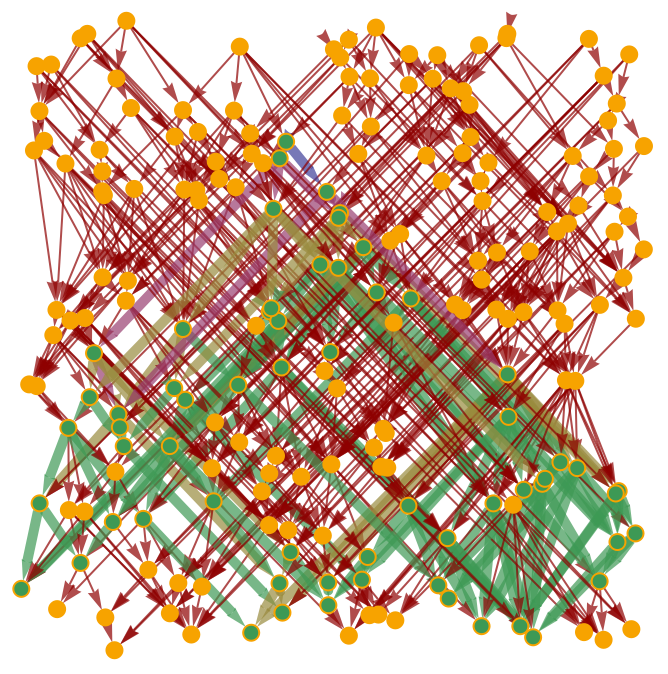
The figure below shows an example of how the Hausdorff dimension is calculated for the exampleCausalGraph at the exampleVertex. The different colours represent different radii starting from the exampleVertex. As expected, we see that following progressively larger radii covers a geodesic cone (which effectively corresponds to the future light cone) up to the point where the boundaries of the graph are reached.
Out[]=
An important point to keep in mind is that even the WolframHausdorffDimension can provide different estimates depending on some options (as is clearly explained in the function documentation). For example, one might calculate the dimension using all possible radii, set a minimum or maximum radius to try to minimize local and boundary effects, respectively. One can also calculate the dimension at a single point or at multiple points, and in the latter case one can still choose whether to pick the minimum, maximum or average across all local estimates. So once again, we see how important it is to be clear about the choices of the estimate being used.
As an example, we now calculate the local dimension at exampleVertex by radius (or causal layer). In this case, we did not select any minimum nor maximum radius, so the calculation will be performed for all possible radii. As such, it is expected that there will be boundary effects affecting the results, especially as the radius becomes closer to the boundary.
As an example, we now calculate the local dimension at exampleVertex by radius (or causal layer). In this case, we did not select any minimum nor maximum radius, so the calculation will be performed for all possible radii. As such, it is expected that there will be boundary effects affecting the results, especially as the radius becomes closer to the boundary.
In[]:=
ResourceFunction["WolframHausdorffDimension"][exampleCausalGraph,exampleVertex,"Dimension","DimensionMethod"->Identity]
Out[]=
{1.58496,2.70951,4.29906,3.03341}
Is is clear that the dimensions calculated when using a different maximum radius are different, and this obviously can have an impact in the results of the calculations performed in this project. Instead of calculating the dimensions at progressively larger radii, we are interested in having a single dimension estimate at the exampleVertex. There are several methods which can be used for this, and for this project we chose to use a Mean over the dimensions calculated above for each radius.
In[]:=
ResourceFunction["WolframHausdorffDimension"][exampleCausalGraph,exampleVertex,"Dimension","DimensionMethod"->Mean]
Out[]=
2.90674
We can do this across all vertices and average the results to obtain an estimate of the global graph dimension:
In[]:=
ResourceFunction["WolframHausdorffDimension"][exampleCausalGraph,All,"AllDimensions","VertexMethod"->Mean]
Out[]=
1.88429
Now, because the causal graph was created by sprinkling, we actually know that its dimension should approach 2. It is interesting how the global dimension estimate is 1.5 and the local dimension estimate at the exampleVertex is 2.7. Simply by enforcing a maximum radius to exclude some boundary effects, e.g. 3, we can change the global estimate.
In[]:=
ResourceFunction["WolframHausdorffDimension"][exampleCausalGraph,All,{1,3},"AllDimensions","VertexMethod"->Mean]
Out[]=
2.14725
Similarly, by selecting a vertex lower down in the causal graph (with boundary effects preventing the light cone from growing as desired) we would expect the local dimension at that vertex to be lower e.g.:
In[]:=
ClearAll[exampleVertex2]exampleVertex2=RandomChoice[Select[VertexList[exampleCausalGraph],Last[#]<0.6&]];ResourceFunction["WolframHausdorffDimension"][exampleCausalGraph,exampleVertex2,"Dimension","DimensionMethod"->Mean]
(Note that by running the code above multiple times, a wide range of local dimensions will be found as the exampleVertex2 moves from one point to another. )
As mentioned above, it is possible to restrict the dimension calculations to include only certain radii, and this may yield better estimates. However, for the purpose of this project we are only interested in the effects of dimension change, and so as long as all dimensions are calculated consistently, it is not as relevant exactly which version of the local estimation is used. However, it is important to keep in mind that the results presented here might change if a different dimension estimate is used.
Dimension perturbation
Dimension perturbation
We saw above that the Wolfram Hausdorff dimension estimate relies on counting the number of vertices which are a certain number of causal edges away. As such, it is possible to perturb the dimension locally by adding or removing edges between a chosen vertex and another vertex connected to it. Since we want to isolate the effect of dimension perturbations, we want to perturb the graph in a way which leaves its causal structure unchanged. In order to do this, we choose to only add edges between pairs of vertices which were already connected by a causal path, and not to remove any edges.
The basic procedure used for the dimension perturbation is to pick an origin vertex, in this case exampleVertex, select another vertex from within its light cone, in this case exampleVertex3, and add an edge to between them to the causal graph. Below we show an example of this procedure.
The basic procedure used for the dimension perturbation is to pick an origin vertex, in this case exampleVertex, select another vertex from within its light cone, in this case exampleVertex3, and add an edge to between them to the causal graph. Below we show an example of this procedure.
We can now assess how this edge addition affected the global and local (at exampleVertex) dimensions of the graph, respectively:
So we see that the addition of this single edge caused a perturbation of the local dimension at the exampleVertex, without significantly altering the global graph dimension. This is the dimension perturbation technique we will use in all the calculations shown in the next section. There are a few points worth mentioning with respect to the edge addition in the remainder of this project:
1. Since we are interested only in how the horismos is affected by dimension changes, for the purpose of this project we only add edges between an origin vertex and a vertex in its horismos (i.e. we do not perform any edge additions to the green points in the figure above, only to the blue ones. This is valid for the coordinate based studies since the definition of the horismos depends only on the vertex coordinates, which do not change with edge additions. However, when studying these effects on non coordinate causal graphs it might be relevant to allow for new edges between any point in the future light cone, as this may change the number of shortest paths to some vertices and hence include/exclude them from the horismos. This was not done in this study.
2. For the purpose of a systematic dimension perturbation study, we choose to perturb the original causal graph by adding all possible edges between the origin vertex and its horismos, one at a time. We tried to add edges between random vertices in the future light cone of the origin vertex, but noticed that these did not produce a significant dimension change at the origin vertex, and so we choose to stick to edges starting from the origin vertex only. For simplicity, we also chose to stick to one edge addition at a time.
Methodology
Methodology
In order to systematically investigate the effect of dimension propagation in the horismos, the following methodology was used:
1) Create a causal graph by sprinkling;
2) Choose a set of origin vertices;
3) Calculate the local dimension of the graph at each of the origin vertices;
4) Modify the causal graph by systematically adding edges to each origin vertex;
5) Calculate the local dimension at each origin for all the new graphs produced by adding edges from that origin;
6) Compare me modified to the original local dimension at the origin vertices;
7) Find the mean position and mean deviation for the original graph by causal layer;
8) Calculate the mean position and mean deviation changes for all the modified graphs, and store them together with the corresponding dimension change for that modified graph;
9) Analyse the results.
The calculations and corresponding key results are presented in the next section, and a detailed explanation of how each of the steps above are implemented in practice is available below.
Key Results
Key Results
Results
Results
Original vs modified local dimensions
Original vs modified local dimensions
The local (WolframHausdorffDimension) dimensions at each origin vertex in the original causal graph (i.e. before any edge additions) are shown below. Note that the local dimensions at the origin vertices are likely to be higher than the global dimension since they are selected on purpose to be far from the lower boundary of the causal graph, resulting in a lack of lower boundary effects, which would otherwise tend to decrease the global dimension.
Below we can see the local dimension change for each of the edge additions (tab1), a histogram of all the dimension changes (tab2) and a zoomed in version of the same histogram, but for the main part of the plot only (tab3).
Positive vs negative dimension changes
Positive vs negative dimension changes
Below we show some analysis that was performed in an attempt to compare the cases which let to a positive vs negative dimension change with respect to the original plots.
We start by investigating how the dimension change depends on the original path length between the vertices connected by the new edge.
Next we investigate how the dimension change depends on the original local plot dimension at the origin vertex of the new added edge.
Finally, we investigate how the dimension change depends on the coordinates of the original plot, in an attempt to test whether there are any obvious boundary effects at play. For simplicity we only look at the time coordinate (tab1) and one of the spatial coordinates(tab2).
Effects of dimension change on the spatial structure of the horismos
Effects of dimension change on the spatial structure of the horismos
Now we move beyond looking at the dimension changes produced by the different perturbations we performed in the original causal graph, and onto investigating how these modifications affect the horismos, where null geodesics propagate, as a function of the dimension changes produced by those perturbations. At this stage, we make use of the fact that the causal graphs used here have coordinate information for the different vertices.
In order to assess these effects, we look at different “causal slices” of the horismos. Each slice consists of the points in the horismos of each origin vertex which are at the same causal distance from the origin vertex, i.e. which are separated from it by the same number of causal edges. In the following analysis we only look at the effects on causal layer 2 and above, and each tab shows the results of the corresponding causal layer .
And below we can see how the way the horismos points in each causal layer deviate from the mean changes after the dimension perturbation.
In order to better quantify whether there is a clear relationship between the dimension change and the average coordinate change (or the average deviation from the mean change), we calculated some correlations between these quantities.This is done by causal layer and here we show them for layer 2 as an example.
Discussion
Discussion
Original local dimensions
Original local dimensions
The first thing that might be noticed when looking at the original local dimensions is their relatively high value compared to the dimension of the original sprinkling. This is due to two things: first, as discussed in the dimension estimation section, we are not setting any lower or upper bounds to the radius to be used in the calculations, which makes the estimate less accurate. As discussed in that section, this is not a problem for the purpose of this work, since we only care about the dimension change, and not the absolute dimension. The same argument is valid for the global dimension of the graph, which does not correspond exactly to the sprinkling dimension.
The second effect is the fact that all the vertices selected as origins purposely have a relatively high time coordinate. This biases the local estimates to higher values. If the local dimensions were performed for a set of vertices with time coordinate e.g. lower than 0.3, the effect would be the opposite and the local dimensions would all be lower, e.g.:
The second effect is the fact that all the vertices selected as origins purposely have a relatively high time coordinate. This biases the local estimates to higher values. If the local dimensions were performed for a set of vertices with time coordinate e.g. lower than 0.3, the effect would be the opposite and the local dimensions would all be lower, e.g.:
Dimension changes
Dimension changes
The results clearly show that the majority of the perturbations by edge addition cause a negative dimension change. We did not find a good fit to the dimension change histogram data which was not a clear over fit. Although the general features of this histogram are constant for different sprinklings, some important ones change (e.g. the skewness of the main part of the histogram), making it harder to come up with a compelling explanation of its detailed shape.
We investigated the conditions which lead to a positive vs negative dimension change by looking at several properties of the added edges. These included the original shortest path connecting the vertices involved, the original local dimension at the origin vertex, and the time and space coordinates of the origin vertex. The results, shown in the Positive vs negative dimension changes section, do not show any clear dependencies. Although we did not reach a clear conclusion here, it is important to understand what is causing these changes, as in future work we might be interested in investigating edge additions which cause only positive or negative dimension changes. It is possible that different local dimension estimators would yield different results with clearer indications of what edges would lead to positive or negative dimension changes. This is an important avenue for future work.
We investigated the conditions which lead to a positive vs negative dimension change by looking at several properties of the added edges. These included the original shortest path connecting the vertices involved, the original local dimension at the origin vertex, and the time and space coordinates of the origin vertex. The results, shown in the Positive vs negative dimension changes section, do not show any clear dependencies. Although we did not reach a clear conclusion here, it is important to understand what is causing these changes, as in future work we might be interested in investigating edge additions which cause only positive or negative dimension changes. It is possible that different local dimension estimators would yield different results with clearer indications of what edges would lead to positive or negative dimension changes. This is an important avenue for future work.
Correlation with spatial coordinates
Correlation with spatial coordinates
The correlations between the dimension change and spatial coordinate measures do not look very promising. This is an indication that, although there are clear changes happening to the horismos (which are visible by the fact that both the mean and mean deviation change in the perturbed graphs) the physical coordinates are probably not the most interesting property of the horismos for the purpose of investigating the effect of dimension change. In fact, since we saw that we can view the edge additions as relabelings of the causal layers of certain vertices, it seems plausible that properties related directly to the causal relations in the horismos might have a clearer dependency on dimension change. If one uses a combinatorics definition of the horismos, it is even possible that the edge additions change which points belong to the horismos, which does not happen when using a coordinate based definition. This might result in more impactful changes which might also be more strongly correlated to the dimension perturbations.
Concluding remarks
Concluding remarks
The results indicate that dimension perturbations have an impact on the shape of the horismos. However, this impact is not obviously quantifiable in terms of mean and mean deviation of spatial coordinates projected onto causal layers. One hypothesis that arises from these studies is that perhaps the effects of dimension variations are clearer with regards to coordinate-independent properties of the horismos. These have two advantages: firstly, they would be directly applicable to causal graphs resulting from the evolution of Wolfram Model; secondly, they might bring to light correlations which are not visible when looking only at coordinate dependent properties. As such, it would be important to use the techniques developed in this work to explore of the effects of dimension perturbations on coordinate independent properties of the horismos.
Regardless of whether or not the chosen horismos properties show an interesting dependence on the local dimension change, with this work we have demonstrated that is it possible to study such effects in a systematic manner. The methodology developed here is general enough that it can be extended to the study of different properties of the horismos, some of which may present clearer dependencies on the dimension change.
The lack of clear correlations between the properties studied in this project leads to one interesting conclusion: if there are spatial lensing-like effects caused by perturbation variations, these do not seem to be straightforward, and more investigation is needed in order to establish them.
Future directions
Future directions
A proposed avenue for an extension of the work shown here would be to come up with interesting coordinate free properties of the horismos and assess the effect that dimension changes have on these. In order to do this, first it will be necessary to fine tune the combinatorics definition of the horismos, as briefly discussed in the horismos section. As a first step, these investigations can be performed on sprinkled causal graphs, even if the coordinate information is not used, which are known to approximate to a certain well behaved manifold - unlike the case of a general causal graph. Also, the tools developed in this project will work for these causal graphs. When generalizing to dynamically grown graphs, some adaptations to the functions presented in this work will be needed, though the overall methodology should still be valid.
Another potential avenue would be to compare the “lensing” effects of dimension perturbations to curvature perturbations. As of now, it is not obvious what the best approach to do this would be. However, it is certainly an important comparison to make, especially if we want to be able to distinguish curvature from dimension perturbation effects in some future experiment.
Another potential avenue would be to compare the “lensing” effects of dimension perturbations to curvature perturbations. As of now, it is not obvious what the best approach to do this would be. However, it is certainly an important comparison to make, especially if we want to be able to distinguish curvature from dimension perturbation effects in some future experiment.
Appendix 1 - Necessary Functions
Appendix 1 - Necessary Functions
Keywords
Keywords
◼
Causal Graph
◼
Sprinkling
◼
Dimension
◼
Horismos
Acknowledgments
Acknowledgments
First and foremost, I would like to thank my mentor Jonathan Gorard for his ongoing availability to discuss this project, both conceptually and technically - even before the summer school had started - and for carefully reading through this document before submission! Secondly, I would like to thank Cameron Beetar for the long conceptual discussions we had about the results of this project and for, together with Jonathan, bringing lots of laughter to these four weeks.
Next, I would like to thank all the people in our mentor group for all the science discussion and for making the summer school so enjoyable - Ariadna Uxue Palomino Ylla, Jan Chojnacki, Julia Dannemann-Freitag, Salvo Vultaggio and Vlad Kuchkin. I would like to thank Stephen Wolfram for the discussion which lead to the choice of this project, for his time in sharing his knowledge with us during this school and for the Q&As he hosted with very interesting people. Finally, I would like to thank Erin Cherry, the TAs and all the admin team for their general availability and for making this school run so smoothly.
Next, I would like to thank all the people in our mentor group for all the science discussion and for making the summer school so enjoyable - Ariadna Uxue Palomino Ylla, Jan Chojnacki, Julia Dannemann-Freitag, Salvo Vultaggio and Vlad Kuchkin. I would like to thank Stephen Wolfram for the discussion which lead to the choice of this project, for his time in sharing his knowledge with us during this school and for the Q&As he hosted with very interesting people. Finally, I would like to thank Erin Cherry, the TAs and all the admin team for their general availability and for making this school run so smoothly.
References
References
◼
[1]: Stephen Wolfram (2020): A Class of Models with the Potential to Represent Fundamental Physics. Complex Syst. 29(2), doi:10.25088/complexsystems.29.2.107. Available at https: //www.complex-systems.com/abstracts/v29_i02_a01/
◼
[2]: Jonathan Gorard (2020): “Algorithmic causal sets and the Wolfram model”. ArXiv preprint available at: https://arxiv.org/abs/2011.12174
◼
[3]: Antonio Masiello, Paolo Piccione (1996): “Shortening null geodesics in Lorentzian manifolds. Applications to closed light rays”. Available at: https://core.ac.uk/download/pdf/82390683.pdf
◼
[4]: David A. Meyer (1988): “The dimension of causal sets”. Available at https://dspace.mit.edu/bitstream/handle/1721.1/14328/21880120-MIT.pdf?sequence=2&isAllowed=y
◼
[5]: WolframHausdorffDimension, documentation page: https://resources.wolframcloud.com/FunctionRepository/resources/WolframHausdorffDimension